Vote Arlington 4: Analyzing the Data

PostGIS proved to be an effective tool in manipulating and processing data into the format needed for analysis. To do that analaysis, however, I’ll turn to Python tools.

From PostGIS to Pandas

The first step is to get the final table at the end of Vote Arlington 3: Processing the Data out of the database and into a pandas DataFrame. A bit of SQLAlchemy will make this a snap:

import pandas as pd
from sqlalchemy import create_engine

connect_str = 'postgresql://jelkner:passwd@localhost:5432/our_arlington'
engine = create_engine(connect_str)
d = pd.read_sql_table('precinct_data', con=engine, index_col='precinct_num')
d.to_pickle('precinct_data.pkl')

Note

passwd here was substituted for the actual database password.

and now I can use NumPy, SciPy and Allen Downey’s thinkstats2.py module in addition to pandas to compute some useful statistics on the data:

import pandas as pd
import matplotlib.pyplot as plt
import numpy as np
import statistics as stat
import thinkstats2 as ts
import thinkplot as tp
import scipy.stats.stats as scistat


# Define a helper function for printing stats
def report_stats(statlist):
    for raw_message, value, value_format in statlist:
        message = raw_message + value_format
        print(message.format(value))
    print()


# Load the data and sort by income
data = pd.read_pickle('Data/precinct_data.pkl')
sd = data.sort_values(by=['income_per_cap'])

# Load the two Series from the DataFrame
income = sd['income_per_cap']
voting = sd['vote_rate']

# Generate scatter plot and least squares line
plt.rcdefaults()
inter, slope = ts.LeastSquares(income, voting)
fit_income, fit_voting = ts.FitLine(income, inter, slope)
tp.Scatter(income, voting)
tp.Plot(fit_income, fit_voting)
tp.Show(title='Voting Rate vs Income in Arlington, VA 2010 Election',
        xlabel='Income per Capita ($)',
        ylabel='Voting Participation Rate (%)')

# Report descriptive statistics on the data
ds = [('Mean income: $', round(stat.mean(income)), '{}'),
      ('Mean voting participation rate: ', round(stat.mean(voting)), '{}%'),
      ('Median income: ', stat.median(income), '${}'),
      ('Median voting participation rate: ', stat.median(voting), '{}%'),
      ('Income sample standard deviation: ', round(stat.stdev(income)), '${}'),
      ('Voting participation rate sample standard deviation: ',
       stat.stdev(voting), '{:0.2f}%')]

report_stats(ds)

# Investigate correlation between income and voting participation
covar = np.cov(income, voting)[0][1]
rho, p_val = scistat.pearsonr(income, voting)

cs = [('Covariance between income and voting is: ', covar, '{:0.2f}'),
      ("The Pearson's correlation between income and voting is: ", rho,
       '{:0.2f}'),
      ('The p-value for this correlation is: ', p_val, '{:0.2e}')]

report_stats(cs)

which generates the plot:

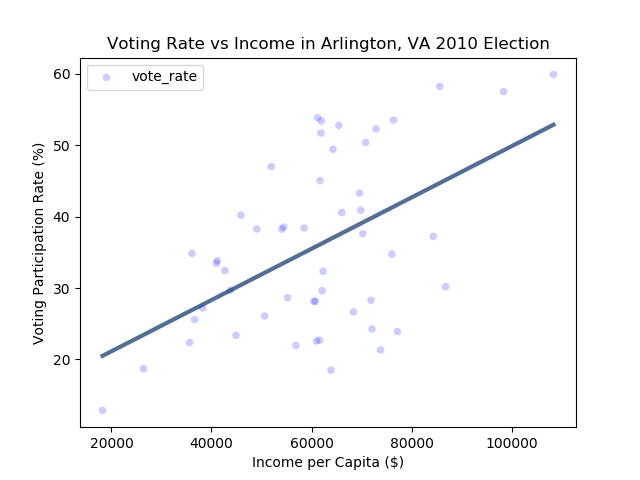
and the following statistics:

Mean income: $60563
Mean voting participation rate: 36.0%
Median income: $61699
Median voting participation rate: 33.83%
Income sample standard deviation: $17310
Voting participation rate sample standard deviation: 12.07%

Covariance between income and voting is: 107588.89
The Pearson's correlation between income and voting is: 0.52
The p-value for this correlation is: 1.10e-04

Results

To reach a conclusion from this process, I defined the null and alternative hypotheses thus:

:math:$H_0$ = There is no correlation between income and voting rate
:math:$H_a$ = There is a positive correlation between income and voting rate

The Pearson’s correlation between income and voting rates in the sample of 51 voting precincts in Arlington County, Virginia in 2010 is 0.52, a borderline high degree of correlation.

The p-value for this correlation is 0.00011, which is well within the statistically highly significant range. The null hypothesis can thus be rejected, and it can be concluded that a correlation between income and voting rate is likely.

Conclusion

I began this investigation began with a hypothesis that I considered likely to hold, that a positive correlation would be found between income and voting participation. In the process of doing the investigation, obtaining and processing the data turned out to be a far greater challenge than the statistical analysis itself. It took a few weeks of investigation (due in large part, no doubt, to my inexperience with this kind of investigation) to find the data sources I needed. It then took an even longer period of time to figure out how to process the data into the format required for analysis. Once that was accomplished, it was a straightforward process to analyze the data and draw a conclusion from it.