7. Classes and objects¶

7.1. Object-oriented programming¶

Python is an object-oriented programming language, which means that it provides features that support object-oriented programming ( OOP).

Object-oriented programming has its roots in the 1960s, but it wasn’t until the mid 1980s that it became the main programming paradigm used in the creation of new software. It was developed as a way to handle the rapidly increasing size and complexity of software systems, and to make it easier to modify these large and complex systems over time.

Up to now we have been writing programs using a procedural programming paradigm. In procedural programming the focus is on writing functions or procedures which operate on data. In object-oriented programming the focus is on the creation of objects which contain both data and functionality together.

7.2. User-defined compound types¶

We will now introduce a new Python keyword, class, which in essence defines a new data type. We have been using several of Python’s built-in types throughout this book, we are now ready to create our own user-defined type: the Point.

Consider the concept of a mathematical point. In two dimensions, a point is two numbers (coordinates) that are treated collectively as a single object. In mathematical notation, points are often written in parentheses with a comma separating the coordinates. For example, (0, 0) represents the origin, and (x, y) represents the point x units to the right and y units up from the origin.

A natural way to represent a point in Python is with two numeric values. The question, then, is how to group these two values into a compound object. The quick and dirty solution is to use a list or tuple, and for some applications that might be the best choice.

An alternative is to define a new user-defined compound type, called a class. This approach involves a bit more effort, but it has advantages that will be apparent soon.

A class definition looks like this:

class Point:
    pass

Class definitions can appear anywhere in a program, but they are usually near the beginning (after the import statements). The syntax rules for a class definition are the same as for other compound statements. There is a header which begins with the keyword, class, followed by the name of the class, and ending with a colon.

This definition creates a new class called Point. The pass statement has no effect; it is only necessary because a compound statement must have something in its body. A docstring could serve the same purpose:

class Point:
    "Point class for storing mathematical points."

By creating the Point class, we created a new type, also called Point. The members of this type are called instances of the type or objects. Creating a new instance is called instantiation, and is accomplished by calling the class. Classes, like functions, are callable, and we instantiate a Point object by calling the Point class:

>>> type(Point)
<class 'type'>
>>> p = Point()
>>> type(p)
<class '__main__.Point'>

The variable p is assigned a reference to a new Point object.

It may be helpful to think of a class as a factory for making objects, so our Point class is a factory for making points. The class itself isn’t an instance of a point, but it contains the machinary to make point instances.

7.3. Attributes¶

Like real world objects, object instances have both form and function. The form consists of data elements contained within the instance.

We can add new data elements to an instance using dot notation:

>>> p.x = 3
>>> p.y = 4

This syntax is similar to the syntax for selecting a variable from a module, such as math.pi or string.uppercase. Both modules and instances create their own namespaces, and the syntax for accessing names contained in each, called attributes, is the same. In this case the attribute we are selecting is a data item from an instance.

The following state diagram shows the result of these assignments:

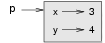
The variable p refers to a Point object, which contains two attributes. Each attribute refers to a number.

We can read the value of an attribute using the same syntax:

>>> print(p.y)
4
>>> x = p.x
>>> print(x)
3

The expression p.x means, “Go to the object p refers to and get the value of x”. In this case, we assign that value to a variable named x. There is no conflict between the variable x and the attribute x. The purpose of dot notation is to identify which variable you are referring to unambiguously.

You can use dot notation as part of any expression, so the following statements are legal:

print('({0}, {1})'.format(p.x, p.y))
distance_squared = p.x * p.x + p.y * p.y

The first line outputs (3, 4); the second line calculates the value 25.

7.4. The initialization method and `self`¶

Since our Point class is intended to represent two dimensional mathematical points, all point instances ought to have x and y attributes, but that is not yet so with our Point objects.

>>> p2 = Point()
>>> p2.x
Traceback (most recent call last):
  File "<stdin>", line 1, in <module>
AttributeError: 'Point' object has no attribute 'x'
>>>

To solve this problem we add an initialization method to our class.

class Point:
    def __init__(self, x, y):
        self.x = x
        self.y = y

A method behaves like a function but it is part of an object. Like a data attribute it is accessed using dot notation.

The initialization method is a special method that is invoked automatically when an object is created by calling the class. The name of this method is __init__ (two underscore characters, followed by init, and then two more underscores). This name must be used to make a method an initialization method in Python.

There is no conflict between the attribute self.x and the parameter x. Dot notation specifies which variable we are referring to.

Let’s add another method, distance_from_origin, to see better how methods work:

class Point:
    def __init__(self, x, y):
        self.x = x
        self.y = y

    def distance_from_origin(self):
        return ((self.x ** 2) + (self.y ** 2)) ** 0.5

Let’s create a few point instances, look at their attributes, and call our new method on them:

>>> p = Point(3, 4)
>>> p.x
3
>>> p.y
4
>>> p.distance_from_origin()
5.0
>>> q = Point(5, 12)
>>> q.x
5
>>> q.y
12
>>> q.distance_from_origin()
13.0
>>> r = Point(0, 0)
>>> r.x
0
>>> r.y
0
>>> r.distance_from_origin()
0.0

When defining a method, the first parameter refers to the instance being created. It is customary to name this parameter self. In the example session above, the self parameter refers to the instances p, q, and r respectively.

7.5. Instances as parameters¶

You can pass an instance as a parameter to a function in the usual way. For example:

def print_point(p):
    print('({0}, {1})'.format(p.x, p.y))

print_point takes a point as an argument and displays it in the standard format. If you call print_point(p) with point p as defined previously, the output is (3, 4).

To convert print_point to a method, do the following:

Indent the function definition so that it is inside the class definition.
Rename the parameter to self.

class Point:
    def __init__(self, x=0, y=0):
        self.x = x
        self.y = y

    def distance_from_origin(self):
        return ((self.x ** 2) + (self.y ** 2)) ** 0.5

    def print_point(self):
        print('({0}, {1})'.format(self.x, self.y))

We can now invoke the method using dot notation.

>>> p = Point(3, 4)
>>> p.print_point()
(3, 4)

The object on which the method is invoked is assigned to the first parameter, so in this case p is assigned to the parameter self. By convention, the first parameter of a method is called self. The reason for this is a little convoluted, but it is based on a useful metaphor.

The syntax for a function call, print_point(p), suggests that the function is the active agent. It says something like, Hey print_point! Here’s an object for you to print.

In object-oriented programming, the objects are the active agents. An invocation like p.print_point() says Hey p! Please print yourself!

This change in perspective might be more polite, but it is not obvious that it is useful. In the examples we have seen so far, it may not be. But sometimes shifting responsibility from the functions onto the objects makes it possible to write more versatile functions, and makes it easier to maintain and reuse code.

7.6. Object-oriented features¶

It is not easy to define object-oriented programming, but we have already seen some of its characteristics:

Programs are made up of class definitions which contain attributes that can be data (instance variables) or behaviors (methods).
Each object definition corresponds to some object or concept in the real world, and the functions that operate on that object correspond to the ways real-world objects interact.
Most of the computation is expressed in terms of operations on objects.

For example, the Point class corresponds to the mathematical concept of a point.

7.7. Time¶

As another example of a user-defined type, we’ll define a class called Time that records the time of day. Since times will need hours, minutes, and second attributes, we’ll start with an initialization method similar to the one we created for Points.

The class definition looks like this:

class Time:
    def __init__(self, hours, minutes, seconds):
        self.hours = hours
        self.minutes = minutes
        self.seconds = seconds

When we call the Time class, the arguments we provide are passed along to init:

>>> current_time = Time(9, 14, 30)
>>> current_time.hours
9
>>> current_time.minutes
14
>>> current_time.seconds
30

Here is a print_time method for our Time objects that uses string formating to display minutes and seconds with two digits.

To save space, we will leave out the initialization method, but you should include it:

class Time:
    # previous method definitions here...

    def print_time(self):
        s = "{0}:{1:02d}:{2:02d}"
        print(s.format(self.hours, self.minutes, self.seconds)

which we can now invoke on time instances in the usual way:

>>> t1 = Time(9, 14, 30)
>>> t1.print_time()
9:14:30
>>> t2 = Time(7, 4, 0)
>>> t2.print_time()
7:04:00

7.8. Optional arguments¶

We have seen built-in functions that take a variable number of arguments. For example, string.find can take two, three, or four arguments.

It is possible to write user-defined functions with optional argument lists. For example, we can upgrade our own version of find to do the same thing as string.find.

This is the original version:

def find(str, ch):
    index = 0
    while index < len(str):
        if str[index] == ch:
            return index
        index = index + 1
    return -1

This is the new and improved version:

def find(str, ch, start=0):
    index = start
    while index < len(str):
        if str[index] == ch:
            return index
        index = index + 1
    return -1

The third parameter, start, is optional because a default value, 0, is provided. If we invoke find with only two arguments, we use the default value and start from the beginning of the string:

>>> find("apple", "p")
1

If we provide a third parameter, it overrides the default:

>>> find("apple", "p", 2)
2
>>> find("apple", "p", 3)
-1

We can rewrite our initialization method for the Time class so that hours, minutes, and seconds are each optional arguments.

class Time:
    def __init__(self, hours=0, minutes=0, seconds=0):
        self.hours = hours
        self.minutes = minutes
        self.seconds = seconds

When we instantiate a Time object, we can pass in values for the three parameters, as we did with

>>> current_time = Time(9, 14, 30)

Because the parameters are now optional, however, we can omit them:

>>> current_time = Time()
>>> current_time.print_time()
0:00:00

Or provide only the first parameter:

>>> current_time = Time(9)
>>> current_time.print_time()
9:00:00

Or the first two parameters:

>>> current_time = Time (9, 14)
>>> current_time.print_time()
9:14:00

Finally, we can provide a subset of the parameters by naming them explicitly:

>>> current_time = Time(seconds = 30, hours = 9)
>>> current_time.print_time()
9:00:30

7.9. Another method¶

Let’s add a method increment, which increments a time instance by a given number of seconds. To save space, we will continue to leave out previously defined methods, but you should always keep them in your version:

class Time:
    # previous method definitions here...

    def increment(self, seconds):
        self.seconds = seconds + self.seconds

        while self.seconds >= 60:
            self.seconds = self.seconds - 60
            self.minutes = self.minutes + 1

        while self.minutes >= 60:
            self.minutes = self.minutes - 60
            self.hours = self.hours + 1

Now we can invoke increment on a time instance.

>>> current_time = Time(9, 14, 30)
>>> current_time.increment(125)
>>> current_time.print_time()
9:16:35

Again, the object on which the method is invoked gets assigned to the first parameter, self. The second parameter, seconds gets the value 125.

7.10. An example with two `Time`s¶

Let’s add a boolen method, after, that takes two time instances and returns True when the first one is chronologically after the second.

We can only convert one of the parameters to self; the other we will call other, and it will have to be a parameter of the method.

class Time:
    # previous method definitions here...

    def after(self, other):
        if self.hours > other.hours:
            return True
        if self.hours < other.hours:
            return False

        if self.minutes > other.minutes:
            return True
        if self.minutes < other.minutes:
            return False

        if self.seconds > other.seconds:
            return True
        return False

We invoke this method on one object and pass the other as an argument:

if time1.after(time2):
    print("It's later than you think.")

You can almost read the invocation like English: If time1 is after time2, then…

7.10.1. Pure functions and modifiers (again)¶

In the next few sections, we’ll write two versions of a function called add_time, which calculates the sum of two Times. They will demonstrate two kinds of functions: pure functions and modifiers, which we first encountered in the Functions chapter.

The following is a rough version of add_time:

def add_time(t1, t2):
    sum = Time()
    sum.hours = t1.hours + t2.hours
    sum.minutes = t1.minutes + t2.minutes
    sum.seconds = t1.seconds + t2.seconds
    return sum

The function creates a new Time object, initializes its attributes, and returns a reference to the new object. This is called a pure function because it does not modify any of the objects passed to it as parameters and it has no side effects, such as displaying a value or getting user input.

Here is an example of how to use this function. We’ll create two Time objects: current_time, which contains the current time; and bread_time, which contains the amount of time it takes for a breadmaker to make bread. Then we’ll use add_time to figure out when the bread will be done. If you haven’t finished writing print_time yet, take a look ahead to Section before you try this:

>>> current_time = Time(9, 14, 30)
>>> bread_time = Time(3, 35, 0)
>>> done_time = add_time(current_time, bread_time)
>>> print_time(done_time)
12:49:30

The output of this program is 12:49:30, which is correct. On the other hand, there are cases where the result is not correct. Can you think of one?

The problem is that this function does not deal with cases where the number of seconds or minutes adds up to more than sixty. When that happens, we have to carry the extra seconds into the minutes column or the extra minutes into the hours column.

Here’s a second corrected version of the function:

def add_time(t1, t2):
    sum = Time()
    sum.hours = t1.hours + t2.hours
    sum.minutes = t1.minutes + t2.minutes
    sum.seconds = t1.seconds + t2.seconds

    if sum.seconds >= 60:
        sum.seconds = sum.seconds - 60
        sum.minutes = sum.minutes + 1

    if sum.minutes >= 60:
        sum.minutes = sum.minutes - 60
        sum.hours = sum.hours + 1

    return sum

Although this function is correct, it is starting to get big. Later we will suggest an alternative approach that yields shorter code.

7.10.2. Modifiers¶

There are times when it is useful for a function to modify one or more of the objects it gets as parameters. Usually, the caller keeps a reference to the objects it passes, so any changes the function makes are visible to the caller. Functions that work this way are called modifiers.

increment, which adds a given number of seconds to a Time object, would be written most naturally as a modifier. A rough draft of the function looks like this:

def increment(time, seconds):
    time.seconds = time.seconds + seconds

    if time.seconds >= 60:
        time.seconds = time.seconds - 60
        time.minutes = time.minutes + 1

    if time.minutes >= 60:
        time.minutes = time.minutes - 60
        time.hours = time.hours + 1

The first line performs the basic operation; the remainder deals with the special cases we saw before.

Is this function correct? What happens if the parameter seconds is much greater than sixty? In that case, it is not enough to carry once; we have to keep doing it until seconds is less than sixty. One solution is to replace the if statements with while statements:

def increment(time, seconds):
    time.seconds = time.seconds + seconds

    while time.seconds >= 60:
        time.seconds = time.seconds - 60
        time.minutes = time.minutes + 1

    while time.minutes >= 60:
        time.minutes = time.minutes - 60
        time.hours = time.hours + 1

This function is now correct, but it is not the most efficient solution.

7.11. Prototype development versus planning¶

So far in this chapter, we’ve used an approach to program development that we’ll call prototype development. We wrote a rough draft (or prototype) that performed the basic calculation and then tested it on a few cases, correcting flaws as we found them.

Although this approach can be effective, it can lead to code that is unnecessarily complicated – since it deals with many special cases – and unreliable – since it is hard to know if we’ve found all the errors.

An alternative is planned development, in which high-level insight into the problem can make the programming much easier. In this case, the insight is that a Time object is really a three-digit number in base 60! The second component is the ones column, the minute component is the sixties column, and the hour component is the thirty-six hundreds column.

When we wrote add_time and increment, we were effectively doing addition in base 60, which is why we had to carry from one column to the next.

This observation suggests another approach to the whole problem – we can convert a Time object into a single number and take advantage of the fact that the computer knows how to do arithmetic with numbers. The following function converts a Time object into an integer:

def convert_to_seconds(time):
    minutes = time.hours * 60 + time.minutes
    seconds = minutes * 60 + time.seconds
    return seconds

Now, all we need is a way to convert from an integer to a Time object:

def make_time(seconds):
    time = Time()
    time.hours = seconds // 3600
    seconds = seconds - time.hours * 3600
    time.minutes = seconds // 60
    seconds = seconds - time.minutes * 60
    time.seconds = seconds
    return time

You might have to think a bit to convince yourself that this technique to convert from one base to another is correct. Assuming you are convinced, you can use these functions to rewrite add_time:

def add_time(t1, t2):
    seconds = convert_to_seconds(t1) + convert_to_seconds(t2)
    return make_time(seconds)

This version is much shorter than the original, and it is much easier to demonstrate that it is correct (assuming, as usual, that the functions it calls are correct).

7.12. Generalization¶

In some ways, converting from base 60 to base 10 and back is harder than just dealing with times. Base conversion is more abstract; our intuition for dealing with times is better.

But if we have the insight to treat times as base 60 numbers and make the investment of writing the conversion functions (convert_to_seconds and make_time), we get a program that is shorter, easier to read and debug, and more reliable.

It is also easier to add features later. For example, imagine subtracting two Times to find the duration between them. The naive approach would be to implement subtraction with borrowing. Using the conversion functions would be easier and more likely to be correct.

Ironically, sometimes making a problem harder (or more general) makes it easier (because there are fewer special cases and fewer opportunities for error).

7.13. Algorithms¶

When you write a general solution for a class of problems, as opposed to a specific solution to a single problem, you have written an algorithm. We mentioned this word before but did not define it carefully. It is not easy to define, so we will try a couple of approaches.

First, consider something that is not an algorithm. When you learned to multiply single-digit numbers, you probably memorized the multiplication table. In effect, you memorized 100 specific solutions. That kind of knowledge is not algorithmic.

But if you were lazy, you probably cheated by learning a few tricks. For example, to find the product of n and 9, you can write n-1 as the first digit and 10-n as the second digit. This trick is a general solution for multiplying any single-digit number by 9. That’s an algorithm!

Similarly, the techniques you learned for addition with carrying, subtraction with borrowing, and long division are all algorithms. One of the characteristics of algorithms is that they do not require any intelligence to carry out. They are mechanical processes in which each step follows from the last according to a simple set of rules.

In my opinion, it is embarrassing that humans spend so much time in school learning to execute algorithms that, quite literally, require no intelligence.

On the other hand, the process of designing algorithms is interesting, intellectually challenging, and a central part of what we call programming.

Some of the things that people do naturally, without difficulty or conscious thought, are the hardest to express algorithmically. Understanding natural language is a good example. We all do it, but so far no one has been able to explain how we do it, at least not in the form of an algorithm.

7.14. Points revisited¶

Let’s rewrite the Point class in a more object- oriented style:

class Point:
    def __init__(self, x=0, y=0):
        self.x = x
        self.y = y

    def __str__(self):
        return '({0}, {1})'.format(self.x, self.y)

The next method, __str__, returns a string representation of a Point object. If a class provides a method named __str__, it overrides the default behavior of the Python built-in str function.

>>> p = Point(3, 4)
>>> str(p)
'(3, 4)'

Printing a Point object implicitly invokes __str__ on the object, so defining __str__ also changes the behavior of print:

>>> p = Point(3, 4)
>>> print(p)
(3, 4)

When we write a new class, we almost always start by writing __init__, which makes it easier to instantiate objects, and __str__, which is almost always useful for debugging.

7.15. Operator overloading¶

Some languages make it possible to change the definition of the built-in operators when they are applied to user-defined types. This feature is called operator overloading. It is especially useful when defining new mathematical types.

For example, to override the addition operator +, we provide a method named __add__:

class Point:
    # previously defined methods here...

    def __add__(self, other):
        return Point(self.x + other.x, self.y + other.y)

As usual, the first parameter is the object on which the method is invoked. The second parameter is conveniently named other to distinguish it from self. To add two Points, we create and return a new Point that contains the sum of the x coordinates and the sum of the y coordinates.

Now, when we apply the + operator to Point objects, Python invokes __add__:

>>>  p1 = Point(3, 4)
>>>  p2 = Point(5, 7)
>>>  p3 = p1 + p2
>>>  print(p3)
(8, 11)

The expression p1 + p2 is equivalent to p1.__add__(p2), but obviously more elegant. As an exercise, add a method __sub__(self, other) that overloads the subtraction operator, and try it out. There are several ways to override the behavior of the multiplication operator: by defining a method named __mul__, or __rmul__, or both.

If the left operand of * is a Point, Python invokes __mul__, which assumes that the other operand is also a Point. It computes the dot product of the two points, defined according to the rules of linear algebra:

def __mul__(self, other):
    return self.x * other.x + self.y * other.y

If the left operand of * is a primitive type and the right operand is a Point, Python invokes __rmul__, which performs scalar multiplication:

def __rmul__(self, other):
    return Point(other * self.x,  other * self.y)

The result is a new Point whose coordinates are a multiple of the original coordinates. If other is a type that cannot be multiplied by a floating-point number, then __rmul__ will yield an error.

This example demonstrates both kinds of multiplication:

>>> p1 = Point(3, 4)
>>> p2 = Point(5, 7)
>>> print(p1 * p2)
43
>>> print(2 * p2)
(10, 14)

What happens if we try to evaluate p2 * 2? Since the first parameter is a Point, Python invokes __mul__ with 2 as the second argument. Inside __mul__, the program tries to access the x coordinate of other, which fails because an integer has no attributes:

>>> print(p2 * 2)
AttributeError: 'int' object has no attribute 'x'

Unfortunately, the error message is a bit opaque. This example demonstrates some of the difficulties of object-oriented programming. Sometimes it is hard enough just to figure out what code is running.

For a more complete example of operator overloading, see Appendix (reference overloading).

7.16. Polymorphism¶

Most of the methods we have written only work for a specific type. When you create a new object, you write methods that operate on that type.

But there are certain operations that you will want to apply to many types, such as the arithmetic operations in the previous sections. If many types support the same set of operations, you can write functions that work on any of those types.

For example, the multadd operation (which is common in linear algebra) takes three parameters; it multiplies the first two and then adds the third. We can write it in Python like this:

def multadd(x, y, z):
    return x * y + z

This method will work for any values of x and y that can be multiplied and for any value of z that can be added to the product.

We can invoke it with numeric values:

>>> multadd(3, 2, 1)
7

Or with Points:

>>> p1 = Point(3, 4)
>>> p2 = Point(5, 7)
>>> print(multadd(2, p1, p2))
(11, 15)
>>> print(multadd(p1, p2, 1))
44

In the first case, the Point is multiplied by a scalar and then added to another Point. In the second case, the dot product yields a numeric value, so the third parameter also has to be a numeric value.

A function like this that can take parameters with different types is called polymorphic.

As another example, consider the method front_and_back, which prints a list twice, forward and backward:

def front_and_back(front):
    import copy
    back = copy.copy(front)
    back.reverse()
    print(str(front) + str(back))

Because the reverse method is a modifier, we make a copy of the list before reversing it. That way, this method doesn’t modify the list it gets as a parameter.

Here’s an example that applies front_and_back to a list:

>>>   myList = [1, 2, 3, 4]
>>>   front_and_back(myList)
[1, 2, 3, 4][4, 3, 2, 1]

Of course, we intended to apply this function to lists, so it is not surprising that it works. What would be surprising is if we could apply it to a Point.

To determine whether a function can be applied to a new type, we apply the fundamental rule of polymorphism: If all of the operations inside the function can be applied to the type, the function can be applied to the type. The operations in the method include copy, reverse, and print.

copy works on any object, and we have already written a __str__ method for Points, so all we need is a reverse method in the Point class:

def reverse(self):
    self.x , self.y = self.y, self.x

Then we can pass Points to front_and_back:

>>>   p = Point(3, 4)
>>>   front_and_back(p)
(3, 4)(4, 3)

The best kind of polymorphism is the unintentional kind, where you discover that a function you have already written can be applied to a type for which you never planned.

7.17. Glossary¶

class¶: A user-defined compound type. A class can also be thought of as a template for the objects that are instances of it.
instantiate¶: To create an instance of a class.
instance¶: An object that belongs to a class.
object¶: A compound data type that is often used to model a thing or concept in the real world.
attribute¶: One of the named data items that makes up an instance.
pure function¶: A function that does not modify any of the objects it receives as parameters. Most pure functions are fruitful.
modifier¶: A function that changes one or more of the objects it receives as parameters. Most modifiers are void.
functional programming style¶: A style of program design in which the majority of functions are pure.
prototype development¶: A way of developing programs starting with a prototype and gradually testing and improving it.
planned development¶: A way of developing programs that involves high-level insight into the problem and more planning than incremental development or prototype development.
object-oriented language¶: A language that provides features, such as user-defined classes and inheritance, that facilitate object-oriented programming.
object-oriented programming¶: A style of programming in which data and the operations that manipulate it are organized into classes and methods.
method¶: A function that is defined inside a class definition and is invoked on instances of that class. :override:: To replace a default. Examples include replacing a default parameter with a particular argument and replacing a default method by providing a new method with the same name.
initialization method¶: A special method that is invoked automatically when a new object is created and that initializes the object’s attributes.
operator overloading¶: Extending built-in operators ( +, -, *, >, <, etc.) so that they work with user-defined types.
dot product¶: An operation defined in linear algebra that multiplies two Points and yields a numeric value.
scalar multiplication¶: An operation defined in linear algebra that multiplies each of the coordinates of a Point by a numeric value.
polymorphic¶: A function that can operate on more than one type. If all the operations in a function can be applied to a type, then the function can be applied to a type.