5. Functions
Human beings are quite limited in their ability hold distinct pieces of information in their working memories. Research suggests that for most people the number of unrelated chunks is about seven. Computers, by contrast, have no difficulty managing thousands of separate pieces of information without ever forgetting them or getting them confused.
Note
See The Magical Number Seven, Plus or Minus Two for more about this facinating topic.
To make it possible for human beings (programmers) to write complex programs that can span thousands of lines of code, programming languages have features that allow programmers to use the power of abstracton to give names to a sequence of instructions and then to use the new names without having to consider the details of the instructions to which they refer.
This chapter discusses functions, one of Python’s language features that support this kind of abstraction.
5.1. Function definition and use
In the context of programming, a function is a named sequence of statements that performs a desired operation. This operation is specified in a function definition. In Python, the syntax for a function definition is:
def NAME( LIST OF PARAMETERS ):
    STATEMENTS
You can make up any names you want for the functions you create, except that you can’t use a name that is a Python keyword. The list of parameters specifies what information, if any, you have to provide in order to use the new function.
There can be any number of statements inside the function, but they have to be
indented from the def.
Function definitions are compound statements, similar to the branching and looping statements we saw in the Conditionals, loops and exceptions chapter, which means they have the following parts:
A header, which begins with a keyword and ends with a colon.
A body consisting of one or more Python statements, each indented the same amount (4 spaces is the Python standard ) from the header.
In a function definition, the keyword in the header is def, which is
followed by the name of the function and a list of
parameters
enclosed in parentheses. The parameter list may be empty, or it may contain any
number of parameters. In either case, the parentheses are required.
5.2. Building on what you learned in high school Algebra
Back in high school Algebera class you were introduced to mathematical functions. Perhaps you were shown a diagram of a “function machine” that looked something like this:
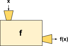
The idea behind this diagram is that a function is like a machine that takes
an input, x, and transforms it into an output, f(x). The light
yellow box f is an abstraction of the process used to do the transformation
from x to f(x).
Functions in Python can be thought of much the same way, and the similarity with functions from Algebra may help you understand them.
The following quadratic function is an example:
f(x) = 3x 2 - 2x + 5
Here is the same function in Python:
def f(x):
    return 3 * x ** 2 - 2 * x + 5
Defining a new function does not make the function run. To do that we need a function call. Function calls contain the name of the function being executed followed by a list of values, called arguments, which are assigned to the parameters in the function definition.
Here is our function f being called with several different arguments:
>>> f(3)
26
>>> f(0)
5
>>> f(1)
6
>>> f(-1)
10
>>> f(5)
70
The function definition must first be entered into the Python shell before it can be called:
>>> def f(x):
...     return 3 * x ** 2 - 2 * x + 5
...
>>>
Function calls involve an implicit assignment of the argument to the parameter
The relationship between the parameter and the argument in the definition
and calling of a function is that of an implicit assignment. It is as if
we had executed the assignment statements x = 3, x = 0, x = 1,
x = -1, and x = 5 respectively before making the function calls
to f in the preceding example.
5.3. The return statement
The return statement causes
a function to immediately stop executing statements in the function body and
to send back (or return) the value after the keyword return to the
calling statement.
>>> result = f(3)
>>> result
26
>>> result = f(3) + f(-1)
>>> result
36
A return statement with no value after it still returns a value, of a type we haven’t seen before:
>>> def mystery():
...    return
...
>>> what_is_it = mystery()
>>> what_is_it
>>> type(what_is_it)
<class 'NoneType'>
>>> print(what_is_it)
None
None is the sole value of Python’s NoneType. We will use it frequently
later on to represent an unknown or unassigned value. For now you need to be
aware that it is the value that is returned by a return statement without
an argument.
All Python function calls return a value. If a function call finishes
executing the statements in its body without hitting a return statement, a
None value is returned from the function.
>>> def do_nothing_useful(n, m):
...     x = n + m
...     y = n - m
...
>>> do_nothing_useful(5, 3)
>>> result = do_nothing_useful(5, 3)
>>> result
>>>
>>> print(result)
None
Since do_nothing_useful does not have a return statement with a value, it
returns a None value, which is assigned to result. None values
don’t display in the Python shell unless they are explicited printed.
Any statements in the body of a function after a return statement is
encountered will never be executed and are referred to as
dead code.
>>> def try_to_print_dead_code():
...    print("This will print...")
...    print("...and so will this.")
...    return
...    print("But not this...")
...    print("because it's dead code!")
...
>>> try_to_print_dead_code()
This will print...
...and so will this.
>>>
5.4. Flow of execution
In order to ensure that a function is defined before its first use, you have to know the order in which statements are executed, which is called the flow of execution.
Execution always begins at the first statement of the program. Statements are executed one at a time, in order from top to bottom.
Function definitions do not alter the flow of execution of the program, but remember that statements inside the function are not executed until the function is called.
Function calls are like a detour in the flow of execution. Instead of going to the next statement, the flow jumps to the first line of the called function, executes all the statements there, and then comes back to pick up where it left off.
That sounds simple enough, until you remember that one function can call another. While in the middle of one function, the program might have to execute the statements in another function. But while executing that new function, the program might have to execute yet another function!
Fortunately, Python is adept at keeping track of where it is, so each time a function completes, the program picks up where it left off in the function that called it. When it gets to the end of the program, it terminates.
What’s the moral of this sordid tale? When you read a program, don’t just read from top to bottom. Instead, follow the flow of execution. Look at this program:
def f1():
    print("Moe")

def f2():
    f4()
    print("Meeny")

def f3():
    f2()
    print("Miny")
    f1()

def f4():
    print("Eeny")

f3()
The output of this program is:
Eeny
Meeny
Miny
Moe
Follow the flow of execution and see if you can understand why it does that.
5.5. Encapsulation and generalization
Encapsulation is the process of wrapping a piece of code in a function, allowing you to take advantage of all the things functions are good for.
Generalization means taking something specific, such as counting the number of digits in a given positive integer, and making it more general, such as counting the number of digits of any integer.
To see how this process works, let’s start with a program that counts the
number of digits in the number 4203:
number = 4203
count = 0

while number != 0:
    count += 1
    number //= 10

print(count)
Apply what you learned in Tracing a program to this until you feel
confident you understand how it works. This program demonstrates an important
pattern of computation called a counter. The variable count is
initialized to 0 and then incremented each time the loop body is executed. When
the loop exits, count contains the result — the total number of times the
loop body was executed, which is the same as the number of digits.
The first step in encapsulating this logic is to wrap it in a function:
def num_digits():
    number = 4203
    count = 0

    while number != 0:
        count += 1
        number //= 10

    return count

print(num_digits())
Running this program will give us the same result as before, but this time we are calling a function. It may seem like we have gained nothing from doing this, since our program is longer than before and does the same thing, but the next step reveals something powerful:
def num_digits(number):
    count = 0

    while number != 0:
        count += 1
        number //= 10

    return count

print(num_digits(4203))
By parameterizing the value, we can now use our logic to count the digits of
any positive integer. A call to print(num_digits(710)) will print 3.
A call to print(num_digits(1345109)) will print 7, and so forth.
This function also contains bugs. If we call num_digits(0), it will return
a 0, when it should return a 1. If we call num_digits(-23), the
program goes into an infinite loop. You will be asked to fix both of these bugs
as an exercise.
5.6. Composition
Just as with mathematical functions, Python functions can be composed, meaning that you use the result of one function as the input to another.
>>> def f(x):
...     return 2 * x
...
>>> def g(x):
...     return x + 5
...
>>> def h(x):
...     return x ** 2 - 3
>>> f(3)
6
>>> g(3)
8
>>> h(4)
13
>>> f(g(3))
16
>>> g(f(3))
11
>>> h(f(g(0)))
97
>>>
We can also use a variable as an argument:
>>> # Assume function definitions for f and g as in previous example
>>> val = 10
>>> f(val)
20
>>> f(g(val))
30
>>>
Notice something very important here. The name of the variable we pass as an
argument (val) has nothing to do with the name of the parameter (x).
Again, it is as if x = val is executed when f(val) is called. It
doesn’t matter what the value was named in the caller, inside f and g
its name is x.
5.7. Functions are data too
The functions you define in Python are a type of data.
>>> def f():
...     print("Hello from function f!")
...
>>> type(f)
<type 'function'>
>>> f()
Hello, from function f!
>>>
Function values can be elements of a list. Assume f, g, and h have
been defined as in the Composition section above.
>>> do_stuff = [f, g, h]
>>> for func in do_stuff:
...     func(10)
...
20
15
97
As usual, you should trace the execution of this example until you feel confident you understand how it works.
5.8. List parameters
Passing a list as an argument actually passes a reference to the list, not a copy of the list. Since lists are mutable changes made to the parameter change the argument as well. For example, the function below takes a list as an argument and multiplies each element in the list by 2:
def double_stuff_v1(a_list):
    index = 0
    for value in a_list:
        a_list[index] = 2 * value
        index += 1
To test this function, we will put it in a file named pure_v_modify.py, and
import it into our Python shell, were we can experiment with it:
>>> from pure_v_modify import double_stuff_v1
>>> things = [2, 5, 'Spam', 9.5]
>>> double_stuff_v1(things)
>>> things
[4, 10, 'SpamSpam', 19.0]
Note
The file containing the imported code must have a .py
file extention, which is
not written in the import statement.
The parameter a_list and the variable things are aliases for the same
object. The state diagram looks like this:
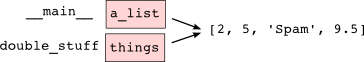
Since the list object is shared by two frames, we drew it between them.
If a function modifies a list parameter, the caller sees the change.
5.9. Pure functions and modifiers
Functions which take lists as arguments and change them during execution are called modifiers and the changes they make are called side effects.
A pure function does not produce side effects. It communicates with the
calling program only through parameters, which it does not modify, and a return
value. Here is double_stuff_v2 written as a pure function:
def double_stuff_v2(a_list):
    new_list = []
    for value in a_list:
        new_list += [2 * value]
    return new_list
This version of double_stuff does not change its arguments:
>>> from pure_v_modify import double_stuff_v2
>>> things = [2, 5, 'Spam', 9.5]
>>> double_stuff_v2(things)
[4, 10, 'SpamSpam', 19.0]
>>> things
[2, 5, 'Spam', 9.5]
>>>
To use the pure function version of double_stuff to modify things,
you would assign the return value back to things:
>>> things = double_stuff(things)
>>> things
[4, 10, 'SpamSpam', 19.0]
>>>
5.10. Which is better?
Anything that can be done with modifiers can also be done with pure functions. In fact, some programming languages only allow pure functions. There is some evidence that programs that use pure functions are faster to develop and less error-prone than programs that use modifiers. Nevertheless, modifiers are convenient at times, and in some cases, functional programs are less efficient.
In general, we recommend that you write pure functions whenever it is reasonable to do so and resort to modifiers only if there is a compelling advantage. This approach might be called a functional programming style.
5.11. Polymorphism and duck typing
The ability to call the same function with different types of data is called polymorphism. In Python, implementing polymorphism is easy, because Python functions handle types through duck typing. Basically, this means that as long as all the operations on a function parameter are valid, the function will handle the function call without complaint. The following simple example illustrates the concept:
>>> def double(thing):
...    return 2 * thing
...
>>> double(5)
10
>>> double('Spam')
'SpamSpam'
>>> double([1, 2])
[1, 2, 1, 2]
>>> double(3.5)
7.0
>>> double(('a', 'b'))
('a', 'b', 'a', 'b')
>>> double(None)
Traceback (most recent call last):
  File "<stdin>", line 1, in <module>
  File "<stdin>", line 2, in double
TypeError: unsupported operand type(s) for *: 'int' and 'NoneType'
>>>
Since * is defined for integers, strings, lists, floats, and tuples,
calling our double function with any of these types as an argument is not
a problem. * is not defined for the NoneType, however, so sending the
double function a None value results in a run time error.
5.12. Two-dimensional tables
A two-dimensional table is a table where you read the value at the intersection of a row and a column. A multiplication table is a good example. Let’s say you want to print a multiplication table for the values from 1 to 6.
A good way to start is to write a loop that prints the multiples of 2, all on one line:
for i in range(1, 7):
    print(2 * i, end="   ")
print()
Here we’ve used the range function, but made it start its sequence at 1.
As the loop executes, the value of i changes from 1 to 6. When all the
elements of the range have been assigned to i, the loop terminates. Each
time through the loop, it displays the value of 2 * i, followed by three
spaces.
Again, the extra end=" " argument in the print function suppresses
the newline, and uses three spaces instead. After the loop completes, the call
to print at line 3 finishes the current line, and starts a new line.
The output of the program is:
2 4 6 8 10 12
So far, so good. The next step is to encapulate and generalize.
5.13. More encapsulation
This function encapsulates the previous loop and generalizes it to print
multiples of n:
def print_multiples(n):
    for i in range(1, 7):
        print(n * i, end="   ")
    print()
To encapsulate, all we had to do was add the first line, which declares the
name of the function and the parameter list. To generalize, all we had to do
was replace the value 2 with the parameter n.
If we call this function with the argument 2, we get the same output as before. With the argument 3, the output is:
3 6 9 12 15 18
With the argument 4, the output is:
4 8 12 16 20 24
By now you can probably guess how to print a multiplication table — by
calling print_multiples repeatedly with different arguments. In fact, we
can use another loop:
for i in range(1, 7):
    print_multiples(i)
Notice how similar this loop is to the one inside print_multiples. All we
did was replace the print function with a function call.
The output of this program is a multiplication table:
1      2      3      4      5      6
2      4      6      8      10     12
3      6      9      12     15     18
4      8      12     16     20     24
5      10     15     20     25     30
6      12     18     24     30     36
5.14. Still more encapsulation
To demonstrate encapsulation again, let’s take the code from the last section and wrap it up in a function:
def print_mult_table():
    for i in range(1, 7):
        print_multiples(i)
This process is a common development plan. We develop code by writing lines of code outside any function, or typing them in to the interpreter. When we get the code working, we extract it and wrap it up in a function.
This development plan is particularly useful if you don’t know how to divide the program into functions when you start writing. This approach lets you design as you go along.
5.15. Local variables
You might be wondering how we can use the same variable, i, in both
print_multiples and print_mult_table. Doesn’t it cause problems when
one of the functions changes the value of the variable?
The answer is no, because the i in print_multiples and the i in
print_mult_table are not the same variable.
Variables created inside a function definition are local; you can’t access a local variable from outside its home function. That means you are free to have multiple variables with the same name as long as they are not in the same function.
Python examines all the statements in a function — if any of them assign a value to a variable, that is the clue that Python uses to make the variable a local variable.
The stack diagram for this program shows that the two variables named i are
not the same variable. They can refer to different values, and changing one
does not affect the other.
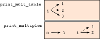
The value of i in print_mult_table goes from 1 to 6. In the diagram it
happens to be 3. The next time through the loop it will be 4. Each time through
the loop, print_mult_table calls print_multiples with the current value
of i as an argument. That value gets assigned to the parameter n.
Inside print_multiples, the value of i goes from 1 to 6. In the
diagram, it happens to be 2. Changing this variable has no effect on the value
of i in print_mult_table.
It is common and perfectly legal to have different local variables with the
same name. In particular, names like i and j are used frequently as
loop variables. If you avoid using them in one function just because you used
them somewhere else, you will probably make the program harder to read.
5.16. Recursive data structures
All of the Python data types we have seen can be grouped inside lists and tuples in a variety of ways. Lists and tuples can also be nested, providing myriad possibilities for organizing data. The organization of data for the purpose of making it easier to use is called a data structure.
It’s election time and we are helping to compute the votes as they come in. Votes arriving from individual wards, precincts, municipalities, counties, and states are sometimes reported as a sum total of votes and sometimes as a list of subtotals of votes. After considering how best to store the tallies, we decide to use a nested number list, which we define as follows:
A nested number list is a list whose elements are either:
numbers
nested number lists
Notice that the term, nested number list is used in its own definition. Recursive definitions like this are quite common in mathematics and computer science. They provide a concise and powerful way to describe recursive data structures that are partially composed of smaller and simpler instances of themselves. The definition is not circular, since at some point we will reach a list that does not have any lists as elements.
Now suppose our job is to write a function that will sum all of the values in a nested number list. Python has a built-in function which finds the sum of a sequence of numbers:
>>> sum([1, 2, 8])
11
>>> sum((3, 5, 8.5))
16.5
>>>
For our nested number list, however, sum will not work:
>>> sum([1, 2, [11, 13], 8])
Traceback (most recent call last):
  File "<stdin>", line 1, in <module>
TypeError: unsupported operand type(s) for +: 'int' and 'list'
>>>
The problem is that the third element of this list, [11, 13], is itself a
list, which can not be added to 1, 2, and 8.
5.17. Recursion
To sum all the numbers in our recursive nested number list we need to traverse the list, visiting each of the elements within its nested structure, adding any numeric elements to our sum, and repeating this process with any elements which are lists.
Modern programming languages generally support recursion, which means that functions can call themselves within their definitions. Thanks to recursion, the Python code needed to sum the values of a nested number list is surprisingly short:
def recursive_sum(nested_num_list):
    the_sum = 0
    for element in nested_num_list:
        if type(element) == list:
            the_sum = the_sum + recursive_sum(element)
        else:
            the_sum = the_sum + element
    return the_sum
The body of recursive_sum consists mainly of a for loop that traverses
nested_num_list. If element is a numerical value (the else branch),
it is simply added to the_sum. If element is a list, then
recursive_sum is called again, with the element as an argument. The
statement inside the function definition in which the function calls itself is
known as the recursive call.
Recursion is truly one of the most beautiful and elegant tools in computer science.
A slightly more complicated problem is finding the largest value in our nested number list:
def recursive_max(nested_num_list):
    """
      >>> recursive_max([2, 9, [1, 13], 8, 6])
      13
      >>> recursive_max([2, [[100, 7], 90], [1, 13], 8, 6])
      100
      >>> recursive_max([2, [[13, 7], 90], [1, 100], 8, 6])
      100
      >>> recursive_max([[[13, 7], 90], 2, [1, 100], 8, 6])
      100
    """
    largest = nested_num_list[0]
    while type(largest) == type([]):
        largest = largest[0]

    for element in nested_num_list:
        if type(element) == type([]):
            max_of_elem = recursive_max(element)
            if largest < max_of_elem:
                largest = max_of_elem
        else:                           # element is not a list
            if largest < element:
                largest = element

    return largest
Doctests are included to provide examples of recursive_max at work.
The added twist to this problem is finding a numerical value for initializing
largest. We can’t just use nested_num_list[0], since that my be either
a number or a list. To solve this problem we use a while loop that assigns
largest to the first numerical value no matter how deeply it is nested.
The two examples above each have a base case which does not lead to a recursive call: the case where the element is a number and not a list. Without a base case, you have infinite recursion, and your program will not work. Python stops after reaching a maximum recursion depth and returns a runtime error.
Write the following in a file named infinite_recursion.py:
#
# infinite_recursion.py
#
def recursion_depth(number):
    print "Recursion depth number %d." % number
    recursion_depth(number + 1)

recursion_depth(0)
At the unix command prompt in the same directory in which you saved your program, type the following:
python infinite_recursion.py
After watching the messages flash by, you will be presented with the end of a long traceback that ends in with the following:
  ...
  File "infinite_recursion.py", line 3, in recursion_depth
    recursion_depth(number + 1)
RuntimeError: maximum recursion depth exceeded
We would certainly never want something like this to happen to a user of one of our programs, so before finishing the recursion discussion, let’s see how errors like this are handled in Python.
5.18. Exceptions
Whenever a runtime error occurs, it creates an exception. The program stops running at this point and Python prints out the traceback, which ends with the exception that occured.
For example, dividing by zero creates an exception:
>>> print 55/0
Traceback (most recent call last):
  File "<stdin>", line 1, in <module>
ZeroDivisionError: integer division or modulo by zero
>>>
So does accessing a nonexistent list item:
>>> a = []
>>> print a[5]
Traceback (most recent call last):
  File "<stdin>", line 1, in <module>
IndexError: list index out of range
>>>
Or trying to make an item assignment on a tuple:
>>> tup = ('a', 'b', 'd', 'd')
>>> tup[2] = 'c'
Traceback (most recent call last):
  File "<stdin>", line 1, in <module>
TypeError: 'tuple' object does not support item assignment
>>>
In each case, the error message on the last line has two parts: the type of error before the colon, and specifics about the error after the colon.
Sometimes we want to execute an operation that might cause an exception, but we
don’t want the program to stop. We can handle the exception using the
try and except statements.
For example, we might prompt the user for the name of a file and then try to open it. If the file doesn’t exist, we don’t want the program to crash; we want to handle the exception:
filename = input('Enter a file name: ')
try:
    f = open(filename, 'r')
except FileNotFoundError:
    print(f'There is no file named {filename}.')
The try statement executes the statements in the first block. If no
exceptions occur, it ignores the except statement. If the file is not
found, a FileNotFoundError is raised. This exception is “caught” by the
except statement and the except branch is executed, and then the
program continues.
We can encapsulate this capability in a function: exists takes a filename
and returns true if the file exists, false if it doesn’t:
def exists(filename):
    try:
        f = open(filename)
        f.close()
        return True
    except:
        return False
You can use multiple except blocks to handle different kinds of exceptions
(see the Errors and Exceptions
lesson from Python creator Guido van Rossum’s Python Tutorial for a more complete discussion of
exceptions).
If your program detects an error condition, you can make it raise an exception. Here is an example that gets input from the user and checks that the number is non-negative.
#
# learn_exceptions.py
#
def get_age():
    age = input('Please enter your age: ')
    if age < 0:
        raise ValueError, '%s is not a valid age' % age
    return age
The raise statement takes two arguments: the exception type, and specific
information about the error. ValueError is the built-in exception which
most closely matches the kind of error we want to raise. The complete listing
of built-in exceptions is found in the Built-in Exceptions section of the Python
Library Reference, again by Python’s creator,
Guido van Rossum.
If the function that called get_age handles the error, then the program can
continue; otherwise, Python prints the traceback and exits:
>>> get_age()
Please enter your age: 42
42
>>> get_age()
Please enter your age: -2
Traceback (most recent call last):
  File "<stdin>", line 1, in <module>
  File "learn_exceptions.py", line 4, in get_age
    raise ValueError, '%s is not a valid age' % age
ValueError: -2 is not a valid age
>>>
The error message includes the exception type and the additional information you provided.
Using exception handling, we can now modify infinite_recursion.py so that
it stops when it reaches the maximum recursion depth allowed:
#
# infinite_recursion.py
#
def recursion_depth(number):
    print "Recursion depth number %d." % number
    try:
        recursion_depth(number + 1)
    except:
        print "Maximum recursion depth exceeded."

recursion_depth(0)
Run this version and observe the results.
5.19. Tail recursion
When the only thing returned from a function is a recursive call, it is referred to as tail recursion.
Here is a version of a function countdown written using tail recursion:
def countdown(n):
    if n == 0:
        print "Blastoff!"
    else:
        print n
        countdown(n-1)
Any computation that can be made using iteration can also be made using
recursion. Here is a version of find_max written using tail recursion:
def find_max(seq, max_so_far):
    if not seq:
        return max_so_far
    if max_so_far < seq[0]:
        return find_max(seq[1:], seq[0])
    else:
        return find_max(seq[1:], max_so_far)
Tail recursion is considered a bad practice in Python, since the Python compiler does not handle optimization for tail recursive calls. The recursive solution in cases like this use more system resources than the equivalent iterative solution.
5.20. Recursive mathematical functions
Several well known mathematical functions are defined recursively. Factorial, for example, is given the special
operator, !, and is defined by:
0! = 1
n! = n(n-1)
We can easily code this into Python:
def factorial(n):
    if n == 0:
        return 1
    else:
        return n * factorial(n-1)
Another well know recursive relation in mathematics is the fibonacci sequence, which is defined by:
fibonacci(0) = 1
fibonacci(1) = 1
fibonacci(n) = fibonacci(n-1) + fibonacci(n-2)
This can also be written easily in Python:
def fibonacci (n):
    if n == 0 or n == 1:
        return 1
    else:
        return fibonacci(n-1) + fibonacci(n-2)
Calling factorial(1000) will exceed the maximum recursion depth. And try
running fibonacci(35) and see how long it takes to complete (be patient, it
will complete).
You will be asked to write an iterative version of factorial as an
exercise, and we will see a better way to handle fibonacci in the next
chapter.
5.21. Glossary
- argument
A value provided to a function when the function is called. This value is assigned to the corresponding parameter in the function.
- flow of execution
The order in which statements are executed during a program run.
- frame
A box in a stack diagram that represents a function call. It contains the local variables and parameters of the function.
- function
A named sequence of statements that performs some useful operation. Functions may or may not take parameters and may or may not produce a result.
- function call
A statement that executes a function. It consists of the name of the function followed by a list of arguments enclosed in parentheses.
- function composition
Using the output from one function call as the input to another.
- function definition
A statement that creates a new function, specifying its name, parameters, and the statements it executes.
- header
The first part of a compound statement. Headers begin with a keyword and end with a colon (:)
- local variable
A variable defined inside a function. A local variable can only be used inside its function.
None¶The sole value of <class ‘NoneType’>.
Noneis often used to represent the absence of a value. It is also returned by areturnstatement with no argument or a function that reaches the end of its body without hitting areturnstatement containing a value.- parameter
A name used inside a function to refer to the value passed as an argument.
- stack diagram
A graphical representation of a stack of functions, their variables, and the values to which they refer.
- traceback
A list of the functions that are executing, printed when a runtime error occurs. A traceback is also commonly refered to as a stack trace, since it lists the functions in the order in which they are stored in the runtime stack.