Dijkstra's Shortest Paths
A Little History
What is the shortest way to travel from Rotterdam to Groningen, in general: from given city to given city. It is the algorithm for the shortest path, which I designed in about twenty minutes. One morning I was shopping in Amsterdam with my young fiancée, and tired, we sat down on the café terrace to drink a cup of coffee and I was just thinking about whether I could do this, and I then designed the algorithm for the shortest path. As I said, it was a twenty-minute invention. In fact, it was published in ’59, three years later. The publication is still readable, it is, in fact, quite nice. One of the reasons that it is so nice was that I designed it without pencil and paper. I learned later that one of the advantages of designing without pencil and paper is that you are almost forced to avoid all avoidable complexities. Eventually, that algorithm became to my great amazement, one of the cornerstones of my fame.
— Edsger Dijkstra, in an interview with Philip L. Frana, Communications of the ACM, 2001.
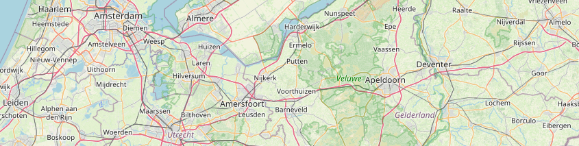
The algorithm to compute the shortest paths from a source node to each of the other nodes was derived by the Dutch computer scientist Edsger Dijkstra in the 1956. He used it in a demonstration program for a new computer called ARMAC. The program contained a graph of 63 Dutch towns connected by roads. A user could input a starting town and a destination town and the computer program would calculate the shortest route through the towns. So, it was basically a Google Maps Driving Directions, version 0.1
The problem is simple if the number of nodes is very small, say five or so. But like the length of a lottery number, each additional node increases possibilities exponentially. At 63 nodes no computer could hope to do this in a simple minded way, even today.
Getting an intuitive sense of the algorithm
Given a network of towns and roads, where the distance between any two adjacent towns along the connecting road is known, Dijkstra's original algorithm computed the shortest path between any two towns in the network. This variation of the algorithm computes the shortest path between a starting node, the source, and all other nodes in the network.
It works by exploring out from the source in a rather unusual way. It is surprisingly fast, especially given that it finds the shortest paths to all of the other nodes more or less at the same time.
Each node has:
- a set of edges that connect it to some of the other nodes
- a path_length, the distance from this node back to the source.
- a state relecting our confidence of the current path_length
Colors are used to denote the state of a node. Blue means the best path to the source has been ascertained, purple denotes that we have a tentative shortest-path, and green denotes that the node has not been visited.
All nodes start out green (unvisited). The source node is the starting point for exploring the netowrk.
To start, the source is immediately assigned to blue with a fixed-path_length of 0. It becomes the current node. (see fig.2 below)
In fact, the current node is the blue node with the shortest path length back to the source.
Now, from the current node, we want to visit only the adjacent nodes that are green (unvisited) or purple (previously visited).
Adding the incremental length between the current node and each neighbor to the current nodes path-length gives us a tentative path_length for the green or purple neighbors.
A green node that has never been visited will be assigned this path_length, and its color is switched to purple.
A purple node will keep the shorter of its tentative path-length of the new one just computed.
After all possible have been visited, we select the one tentative node with the shortest path_length to the source. We set it to blue and make it the current node. It is critical that we select the one with the shortest tentative path. That one and only that one may be safely promoted to fixed.
We repeat our explorations from the new current node and continue until all the nodes are blue.
In figure 7 you can see the the first tentative distance to the source was 66 (coming via A) and later overridden to 65 when coming through B turned out to be shorter.
To get a better sense of how the algorithm works, we will examine this in more detail. The images below were selected from an animation which you can also view.


S is our source node and is set to blue. All the other nodes are still in green. S is our first current-node. Its distance to itself is zero (Shown as S-0)
From S we have visited its neighbors A and B. They are set to purple with tentative distances equal to the edge distance connecting them to S. The computations are “46+0” and “55+0”


Now since A is closer to the source than B, it is chosen as the next current node. Tentative distances to C and D are computed and these are set to purple. Each distance is 66. (46+20). Node A becomes fixed and set to blue
Next, node B is the closest tentative. It goes blue, looks at neighbor C and sees that it can provide it shorter distance back to the source. (65 instead of 66) it updates node C to 65. This is a key step.


Coming into the home stretch now. Node C is now the closest and is set to blue. It has no green or orange neighbors so there is nothing to do.
Finally, node D is likewise dispatched and we are done. The graph is complete with every node blue with its final distance to the source fixed. From any node just follow the blue path back to the source.
To see these changes in action, click here for a javascript animation ![]() . Later our Python program will produce similar animations.
. Later our Python program will produce similar animations.
The Code
The program dijkstra.py may be run in plot mode or in text mode. The text mode keeps things pretty simple and is especially useful for testing as the program is developed. The plot mode uses our now-standard Zelle graphics package.
The program code shown below is available in this zip file.
The attributes of a class Node instance are its…
- position (x,y) in pixels,
- name (uppercase),
- tentative or fixed distance from the source node (or maxint if green),
- a list of adjacent neighbors (other nodes),
- the previous node in the best path (so far) back to the source node,
- its state 0, 1 or 2 corresponding to its color.
At the start of the computation the state of every node is 0. green And when the process completes, the state of every node is 2. blue.
In state 0, the distance to the source node is set as high as possible. sys.maxint is the largest integer value for the word size of your computer. When a node is first set to state 1, the distance will be shortened.
The nbrs list is actually composed of tuples with the 1st item a reference to an adjacent node and the 2nd item the length of the connecting edge. This forms a double link. If node A is a neighbor of node B then node B is also a neighbor of A.
Here is how we define Node instances.
dijkstra.py / class Node
09 class Node :
10     def __init__ (self, name, pos, nbrs=[]) :
11         self.name = name
12         self.pos  = pos
13         self.nbrs = []        # list of neighbor nodes and distance (tuples)
14         self.reset()
15
16     def reset(self) :
17         self.srcDist = maxint # tentative distance to source unknown
18         self.prev = None      # 1st node going back to source
19         self.state = 0        # distance is 0=unknown, 1=tentative or 2=fixed
20
21     def __str__(self) :
22         nbrs = [nbr.name  for nbr,dist in self.nbrs]
23         return "%s: %s" % (self.name, nbrs)
24
Let us look at how the graph is created. A module that contains a function makeGraph() is imported by main in dijkstra.py. This is how our simple example was built.
- Function makeGraph() takes the class definition for Node and creates a list of nodes on the fly. (lines 4-9).
- It also creates a dictionary nodeDict to access to access nodes by their name.
- Variable edges is a list of edges between nodes and is used in the for loop to create the nbrs (neighbors) list in Node pairs. (lines 22-26).
- When finished, the function returns both the list and dictionary of completed nodes.
graph_1.py / makeGraph(Node)
03 def makeGraph (Node) :
04     nodeList = [
05       Node("S", (150, 50)),
06       Node("A", ( 50,150)),
07       Node("B", (200,200)),
08       Node("C", (150,230)),
09       Node("D", ( 50,250))]
10
11     nodeDict = {}
12     for node in nodeList :
13         nodeDict[node.name] = node
14
15     edges = [
16       ("S","A",46),
17       ("S","B",55),
18       ("A","C",20),
19       ("A","D",20),
20       ("B","C",10)]
21
22     for nam1,nam2,incDist in edges :
23         nod1 = nodeDict[nam1]
24         nod2 = nodeDict[nam2]
25         nod1.nbrs.append( (nod2,incDist) )
26         nod2.nbrs.append( (nod1,incDist) )
27
28     return nodeList, nodeDict
dijkstra.py / findPaths(display, nodes, source)
The function findPaths() is at the heart of the program. For now, ignore calls to the function display() and the setting of variables banner and action.
25 def findPaths(display, nodes, source) :  # node names
26     "implements the dijkstra algorithm. Updates nodes dist & prev attributes"
27     for node in nodes : node.reset()
28     source.srcDist = 0
29     source.state   = 1
30     display("Initial Configuration", nodes)
31     while True :
32         best = maxsize; hub = None
33         for test in nodes :
34             if test.state != 2 and test.srcDist < best :
35                 best = test.srcDist
36                 hub  = test
37         if not hub : break                # all nodes in final state
38         hub.state = 2                     # set hub as final
39         display("Node "+hub.name+" set to fixed state",nodes)
40         for nbr,incDist in hub.nbrs :
41             if nbr.state == 2 : continue  # already finalized
42             if nbr.prev == hub: continue  # no looking back !
43             if hub.srcDist+incDist < nbr.srcDist :
44                 if nbr.state == 0 : action = "sets tentative distance to"
45                 else              : action = "overrides distance to"
46                 nbr.state = 1  # tenative capture
47                 nbr.srcDist  = hub.srcDist+incDist
48                 nbr.prev  = hub
49             else :
50                 action = "can't improve distance to source"
51             banner = "%s %s %s" % (hub.name,action,nbr.name)
52             display(banner,nodes)
53     display("Shortest Paths from %s" % source.name, nodes)
54
Function findPaths() is passed a display() function, a list of all the nodes in the graph and the source node.
- Initializaion is done in lines 27-29. All nodes are reset and the source node is set up to get things going.
- The main loop starts at line 31.
- A hub node in sought.
- The hub will be in state 1 and have the smallest tentative distance to the source.
- On the first pass through the loop this will be the source node itself.
- While testing the candidates in the loop at line 33, the variable hub tracks the node with the shortest distance back to the source so far.
- If no hub node is found, we are done.
- Otherwise the hub node is promoted to state 2 (line 38).
- Its neighbors are scanned (line 40) and those that are new or tentative will have their best distance to source (line 47) set.
- New nodes also have their status set to tentative (1).
Displaying Results
The program, dijkstra.py, can be run in either a text or graphic mode. The variable display below points to the appropriate function. The code below produces text output…
displayText.py / display_frame (banner, nodes)
 3 from sys  import maxsize
 4 fig = 0
 5
 6 def display_frame (banner, nodes) :
 7     global fig
 8     fig += 1
 9     print("Fig %d:  %s" % (fig,banner))
10     for node in nodes :
11         dist = node.srcDist
12         if dist == maxsize : dist = "Unknown"
13         print("  %s  state=%s  toSource=%s" % (node.name,node.state,dist))
14
15 def display_close() :
16     pass
17
Below is the (partial) output from the code above.
$ python dijkstra.py graph=graph_1 output=text source=S
..
Fig 2:  Node S set to fixed state
  S  state=2  toSource=0
  A  state=0  toSource=Unknown
  B  state=0  toSource=Unknown
  C  state=0  toSource=Unknown
  D  state=0  toSource=Unknown
Fig 3:  S sets tentative distance to A
  S  state=2  toSource=0
  A  state=1  toSource=46
  B  state=0  toSource=Unknown
  C  state=0  toSource=Unknown
  D  state=0  toSource=Unknown
...
Fig 9:  B overrides distance to C
  S  state=2  toSource=0
  A  state=2  toSource=46
  B  state=2  toSource=55
  C  state=1  toSource=65
  D  state=1  toSource=66
Fig 10:  Node C set to fixed state
  S  state=2  toSource=0
  A  state=2  toSource=46
  B  state=2  toSource=55
  C  state=2  toSource=65
  D  state=1  toSource=66
...
Fig 12:  Shortest Paths from S
  S  state=2  toSource=0
  A  state=2  toSource=46
  B  state=2  toSource=55
  C  state=2  toSource=65
  D  state=2  toSource=66
To get a slide show, you can use the same command but set output=plot…
$ python dijkstra.py graph=graph_1 output=plot source=S
This is the version for displaying graphics output. Though fairly long, it is easy to understand once you have watched it run.
As with the other graphics projects, the Point, Text, and Line objects are drawn and the frame displayed. Before returning it waits for you to click the mouse in the frame. A new frame "undraws" and discards objects from the previous frame before drawing its own.
displayPlot.py
 3 from graphics import *
 4 from sys  import maxsize
 5
 6 colors= ("red","green","blue","orange","yellow","purple")
 7 ncolors = len(colors)
 8
 9 win = GraphWin("Dijkstra's Shortest Paths",400,400)
10 drawn = []
11
12 fig = 0
13
14 def display_clear() :
15     for obj in drawn : obj.undraw()
16
17 def display_frame (banner, nodes) :
18     global fig
19     display_clear()
20     fig += 1
21     banner = "Fig %d:  %s" % (fig,banner)
22     txtBanner = Text(Point(200,20), banner)
23     txtBanner.draw(win)
24     drawn.append(txtBanner)
25
26     display_edges(nodes)
27     display_nodes(nodes)
28     win.getMouse()
29
30 def display_edges(nodes) :
31     edges = {}
32     for node in nodes :
33         for nbr,dist in node.nbrs :
34             tag = tuple(sorted((node.pos,nbr.pos)))  # same edge seen twice
35             state,dist = edges.get(tag, (0,dist)) # white line
36             if nbr.prev == node : state = node.state
37             edges[tag] = state, dist
38
39     for tag in edges :
40         start,end = tag      # split start/end positions
41         state,dist = edges[tag]
42         color = colors[state]
43         p1 = Point(start[0], start[1])
44         p2 = Point(end[0], end[1])
45         line = Line(p1,p2)
46         line.setFill(color)
47         line.draw(win)
48         drawn.append(line)
49
50         mid = ((start[0]+end[0])/2, (start[1]+end[1])/2)
51         txtDist = Text(Point(mid[0],mid[1]), str(dist))
52         txtDist.draw(win)
53         drawn.append(txtDist)
54
55 def display_nodes(nodes) :
56     for node in nodes :
57         color = colors[node.state]
58         label = "%s--%d" % (node.name,node.srcDist)
59         if node.srcDist == maxsize: label = "%s" % node.name
60         x,y = node.pos
61         txtNode = Text(Point(x,y), label)
62         txtNode.setFill(color)
63         txtNode.draw(win)
64         drawn.append(txtNode)
65
66 def display_close() :
67     win.close()
68
main()
The function main() sets the source and output variables. It builds a graph (see below) and then choses the display function for plot or text. findPaths is called and when done the display is closed.
   # dijskstra.py
55 def main()  :
56     srcNode = sarg.Str("source","S")    # default
57     output  = sarg.Str("output","plot")
58     nodes, nodeDict = graph.makeGraph(Node)
59     if output == "plot" :
60         from displayPlot import display_frame, display_close
61     else :
62         from displayText import display_frame, display_close
63     findPaths(display_frame, nodes, nodeDict[srcNode])
64     display_close()
65
66 if __name__ == "__main__" : main()
You can run these with commands like
  $ python dijkstra.py graph=graph_1  # this plots in Zelle graphics
  $ python dijkstra.py graph=graph_2 output=plot # text output
You can download the zip file for dijkstra here
If you have comments or suggestions You can email me at mail me
Copyright © 2014-2021 Chris Meyers and Fred Obermann
* * *