Visualizing Chaos

In school I learned that a population of creatures would grow exponentially unless inhibited by outside factors such as predators or lack of food. For example, bacteria divide and double their population each generation. Since they divide a few times each hour, the population can quickly explode.

But if the creatures are consumed by predators they might be held in check. If not, the predator population might itself boom with such a free lunch. Or the creatures might simply run short on (or even out of) their own food.

More complicated creatures don't divide in each generation but populations will in general grow at a rate K per unit of time. For bacteria that might be 2 per 20 minutes.

We were taught to expect that the situation should stabilize to a natural balance of predator and prey, an equilibrium where the populations reach a steady state. Or perhaps oscillate around some steady point. Whenever things go really hay-wire we expect there to be an extra outside influence (often people) that caused it. Remove the outside influence and the steady state should return.

It turns out that this is quite wrong.

How could anything this simple create such chaos?

I found this equation again after many years in Ian Stewart's "17 equations that changed the world". It is number 16, at least in my German edition. Each value of x (representing a population) generates its successor xs by the operation

xs <- x * (1-x) * k

The k is held constant for a given sequence. The value of x is a real number and between 0 and 1. At zero the population has died out. As we'll see, the equality (0 < x < 1) holds for successors as long as k is confined to a domain of roughly (1 < k < 4).

The equation can simulate a simple population growth and decline where x is a given population and k represents the growth possible in each generation, given no predators or scarcity in food supply. The term (1-x) introduces the brake on the growth. If x is quite small then successors are x times k yielding exponential growth. But then (1-x) quickly increases and puts the damper on this.

What I find very unexpected is that for different domains of k there are clear areas of steady state, oscillatory states, and something new, deterministic chaos. With an incredibly simple Python program we can explore all of this.

Click here to access the first bit of code. It get's the floating point values for k and for an initial x and then proceeds to print out the first 300 successors.

1 # chaos-1.py
2
3 import sys
4 k = float(sys.argv[1])
5 x = float(sys.argv[2])
6 for i in range(30) :
7     print("%.06f" % x)
8     x = x * (1.0-x) * k
9

Let's run this program for various values of K. For K at 1.5 and a starting x value of .2 (which we'll maintain) successive values of x settle into a steady state value of interestingly 1/3.

#                    K   x
$ python chaos-1.py 1.5 .2
0.200000   (our initial x)
0.240000
0.273600
0.298115
0.313863
0.323030
0.328022
0.330636
0.331974
0.332651
0.332991
0.333162
0.333248
0.333291
0.333312
0.333323
0.333328
0.333331
0.333332
0.333333   (x arrives at a steady state value)
0.333333
0.333333

For a higher value of K (3.4) the system settles into oscilation between 2 values .842154 and .451963

$ python chaos-1.py 3.4 .2
0.200000
0.544000
0.843418
0.449019
...
0.841163   (after about 300 steps)
0.842154   (cycle start)
0.451963
0.842154   (cycle start)
0.451963
0.842154   (cycle start)
0.451963

Increasing K from 3.4 to 3.5 makes the system move between 4 values

$ python chaos-1.py 3.5 .2
0.200000
0.560000
0.862400
...
0.500884  (start of cycle)
0.874997
0.382820
0.826941
0.500884  (start of cycle)
0.874997
0.382820

And taking K just a bit further gets us to 8. Notice that we double each time. These are bifurcations and we'll see them more graphically below.

$ python chaos-1.py 3.55 .2
0.200000
0.568000
0.871085
...
0.506031  (start of cycle)
0.887371
0.354800
0.812656
0.540475
0.881684
0.370326
0.827805
0.506031  (start of cycle)
0.887371
0.354800

But at K=3.6 the system does not settle down and after 300 steps we are still in the realm of deterministic chaos.

$ python chaos-1.py 3.6 .2
0.200000
0.576000
0.879206
...
0.789226   (after 300 steps or so)
0.598855
0.864820
0.420864
0.877455
0.387100
0.854113
0.448574

Using PyPlot to Visualize Chaos

If you don't already have matplotlib you will need to install it to follow along with this example. Below is an interactive dialog that demonstrates how we're using it.

>>> import matplotlib.pyplot as plt             # import a plotter
>>> plt.suptitle("This is the title", size=16)  # set upper title
>>> xvals = range(10)                           # make list of x values
>>> xvals
[0, 1, 2, 3, 4, 5, 6, 7, 8, 9]
>>> yvals = [x**2 for x in xvals]               # make list of y values
>>> yvals
[0, 1, 4, 9, 16, 25, 36, 49, 64, 81]
>>> plt.plot(xvals, yvals, 'r')                 # plot x,y in red
>>> plt.show()                                  # Output plot via TK

We use two lists for the x and y values to plot. In this example we just make plot a single quadratic curve in red ('r'). This is what we get in a separate TK window.

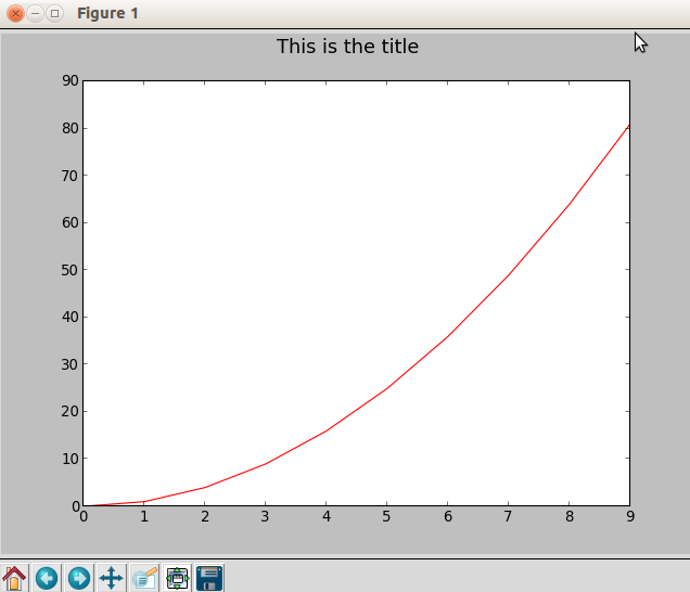
The matplotlib.pyplot is fairly easy to use. It automatically adjusts the view to the range and domain of the x and y lists and even labels the axis for us.

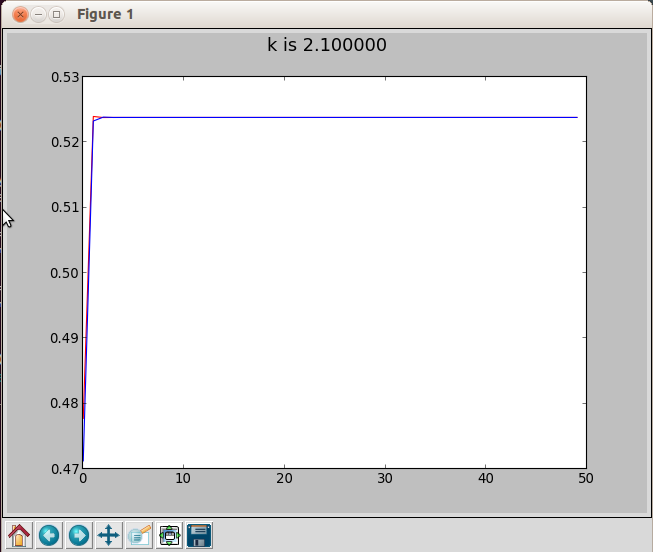
Our program chaos-2.py generates just 50 steps at a given value of K. It actually makes two plots, one in red with an initial x of .35 and one in blue with an initial x of .34. Two plots proceeding from close (but not identical) x values will demostrate a very important aspect of deterministic chaos.

Running chaos-2.py with K at 2.1 gives us an almost immediate steady state in both the red and blue plots. Where the red and blue values are the same, you see only the blue because it is the last one plotted.

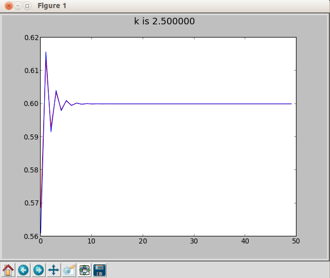
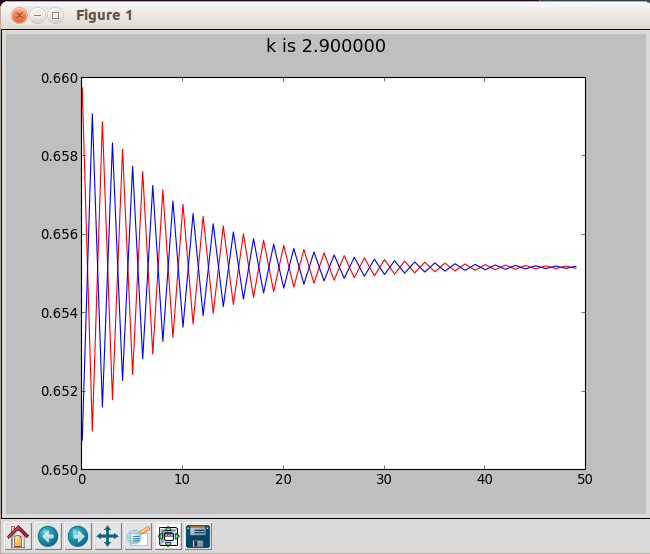
With K at 2.5 a steady state at about .63 is also quickly reached but only after some initial oscillation and some difference between the red and blue plots. K at 2.9 is fun since the red and blue start out almost directly out of sync before reaching the same steady state value.

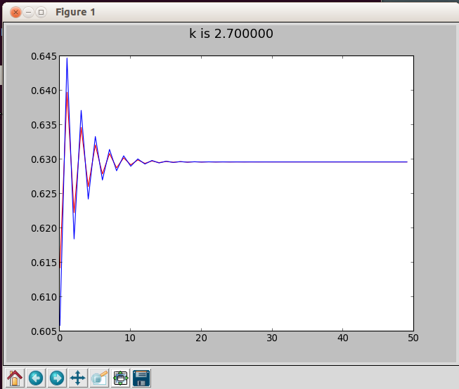
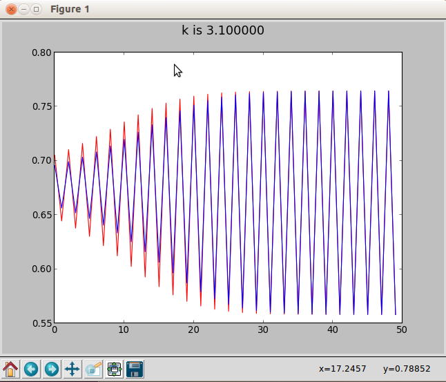
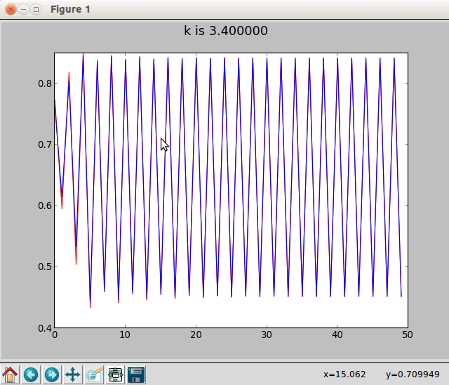
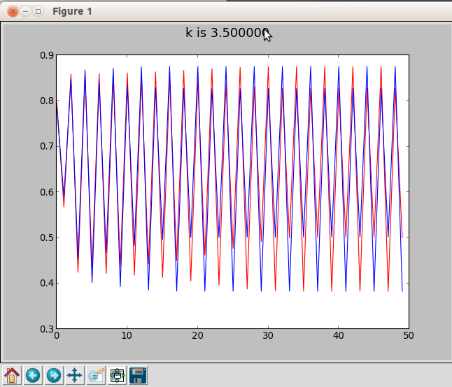
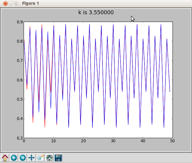
The following plots stabilize into oscillatory behavior. At K=3.1 and K=3.4 both red and blue plots settle into the same 2 value oscillation and also stay in sync. At 3.5 both are in a four value cycle, directly out of sync. At 3.55 we have an 8 value cycle. You have to look a bit carefully to see that it's not four. And red and blue are back in sync.

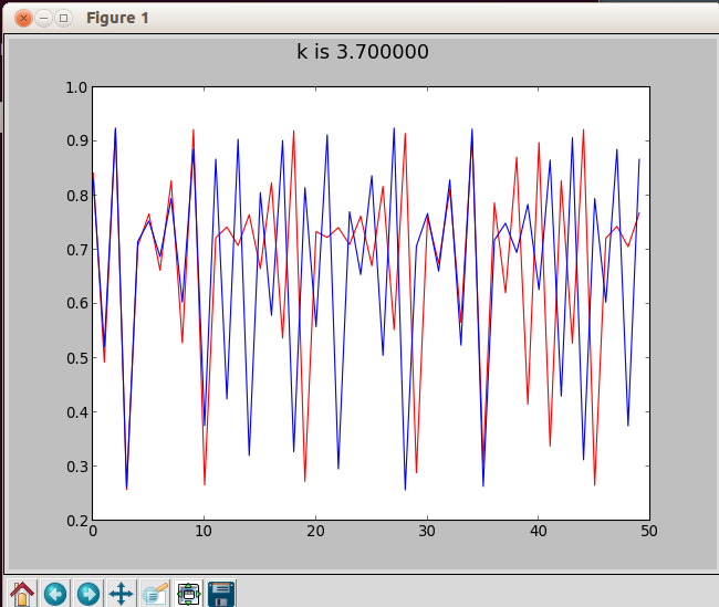
But at K =3.7 we have entered the region of deterministic chaos. We're seeing a graph of surprising growth and collapse. Blue and red start out together but drift apart until at about step 12 they become basically uncoupled.

This demonstrates a very feature of deterministic chaos. The sensitivity to initial conditions" sometimes called the "butterfly effect". It's why we have no hope of accurate weather predictions beyond a range of, currently, 10 days or so.

The Feigenbaum bifurcation diagram

Finally, there is another way to get a rather wonderful overview of the whole system. We can make essentially a scatter plot. For increasing K values (horizontal axis) we generate a set of successors and mark them vertically in a column a pixel wide. Prior to entering chaos when we in oscillation we'll see just one or two (or four or eight or ...) points on any vertical slice of the graph. Then all chaos breaks loose. This is called the Feigenbaum bifurcation diagram.

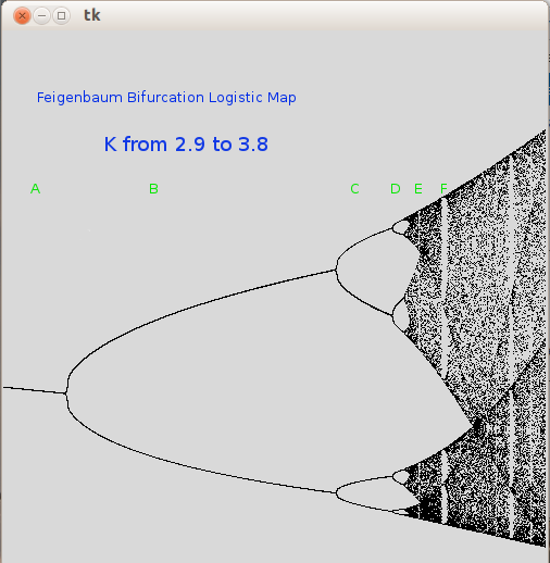
There's a lot going on here. Things change dramatically in different areas that are labeled in green.

On the left (Area A) we are in a steady state where the successor values slowly get smaller as k increases. Then suddenly in area B there is a bifuraction to a 2 value oscillation. As K continues to increase difference between the 2 values increases. Then there is a double bifuration to 4 values (Area C). Eight (Area D) and deterministic chaos. (Area E).

What I find so surprising is how regular it is. The bifurcations form quadratic like curves that "survive" into the chaos as either value boundaries or just areas of increased density of points. Suddenly chaos can turn off temporarily (Area F) and then back on again. And although not shown in the above diagram, when K exceeds 4 the entire system collapses.

I tried to use pyPlot for this but the results were not good. The program that created this graph is chaos-3.py and uses the TK interface directly.

The 3 small programs have been adapted to work fine on both Python 2.7 and any Python 3 version. Of course, Tk must be installed for whichever you use. If you have run other graphic projects that use the John Zelle graphics.py then you already have Tk.

The image was post-edited with GIMP to add the labels and area indicators.

You can download the zip file for the project here.

If you have comments or suggestions You can email me at mail me

* * *