10. Recursion and Exceptions

10.1. Tuples and mutability

So far, you have seen two compound types: strings, which are made up of characters; and lists, which are made up of elements of any type. One of the differences we noted is that the elements of a list can be modified, but the characters in a string cannot. In other words, strings are immutable and lists are mutable.

A tuple, like a list, is a sequence of items of any type. Unlike lists, however, tuples are immutable. Syntactically, a tuple is a comma-separated sequence of values. Although it is not necessary, it is conventional to enclose tuples in parentheses:

>>> julia = ("Julia", "Roberts", 1967, "Duplicity", 2009, "Actress", "Atlanta, Georgia")

Tuples are useful for representing what other languages often call records — some related information that belongs together, like your student record. There is no description of what each of these fields means, but we can guess. A tuple lets us “chunk” together related information and use it as a single thing.

Tuples support the same sequence operations as strings and lists. The index operator selects an element from a tuple.

>>> julia[2]
1967

But if we try to use item assignment to modify one of the elements of the tuple, we get an error:

>>> julia[0] = 'X'
TypeError: 'tuple' object does not support item assignment

Of course, even if we can’t modify the elements of a tuple, we can make a variable reference a new tuple holding different information. To construct the new tuple, it is convenient that we can slice parts of the old tuple and join up the bits to make the new tuple. So julia has a new recent film, and we might want to change her tuple:

>>> julia = julia[:3] + ("Eat Pray Love", 2010) + julia[5:]
>>> julia
('Julia', 'Roberts', 1967, 'Eat Pray Love', 2010, 'Actress', 'Atlanta, Georgia')

To create a tuple with a single element (but you’re probably not likely to do that too often), we have to include the final comma, because without the final comma, Python treats the (5) below as an integer in parentheses:

>>> tup = (5,)
>>> type(tup)
<class 'tuple'>
>>> x = (5)
>>> type(x)
<class 'int'>

10.2. Tuple assignment

Python has a very powerful tuple assignment feature that allows a tuple of variables on the left of an assignment to be assigned values from a tuple on the right of the assignment.

(name, surname, birth_year, movie, movie_year, profession, birth_place) = julia

This does the equivalent of seven assignment statements, all on one easy line. One requirement is that the number of variables on the left must match the number of elements in the tuple.

Once in a while, it is useful to swap the values of two variables. With conventional assignment statements, we have to use a temporary variable. For example, to swap a and b:

temp = a
a = b
b = temp

Tuple assignment solves this problem neatly:

(a, b) = (b, a)

The left side is a tuple of variables; the right side is a tuple of values. Each value is assigned to its respective variable. All the expressions on the right side are evaluated before any of the assignments. This feature makes tuple assignment quite versatile.

Naturally, the number of variables on the left and the number of values on the right have to be the same:

>>> (a, b, c, d) = (1, 2, 3)
ValueError: need more than 3 values to unpack

10.3. Tuples as return values

Functions can return tuples as return values. This is very useful — we often want to know some batsman’s highest and lowest score, or we want to find the mean and the standard deviation, or we want to know the year, the month, and the day, or if we’re doing some some ecological modelling we may want to know the number of rabbits and the number of wolves on an island at a given time. In each case, a function (which can only return a single value), can create a single tuple holding multiple elements.

For example, we could write a function that returns both the area and the circumference of a circle of radius r:

def f(r):
    """ Return (circumference, area) of a circle of radius r """
    c = 2 * math.pi * r
    a = math.pi * r * r
    return (c, a)

10.4. Drawing Fractals

Recursion means “defining something in terms of itself” usually at some smaller scale, perhaps multiple times, to achieve your objective. For example, we might say “A human being is someone whose mother is a human being.”

For our purposes, a fractal is drawing which also has self-similar structure, where it can be defined in terms of itself.

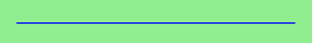
Let us start by looking at the famous Koch fractal. An order 0 Koch fractal is simply a straight line of a given size.

An order 1 Koch fractal is obtained like this: instead of drawing just one line, draw instead four smaller segments, in the pattern shown here:

Now what would happen if we repeated this Koch pattern again on each of the order 1 segments? We’d get this order 2 Koch fractal:

Repeating our pattern again gets us an order 3 Koch fractal:

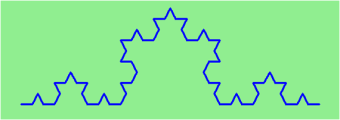
Now let us think about it the other way around. To draw a Koch fractal of order 3, we can simply draw four order 2 Koch fractals. But each of these in turn needs four order 1 Koch fractals, and each of those in turn needs four order 0 fractals. Ultimately, the only drawing that will take place is at order 0. This is very simple to code up in Python:

 def koch(t, order, size):
     """
        Make turtle t draw a Koch fractal of 'order' and 'size'.
        Leave the turtle facing the same direction.
     """

     if order == 0:                  # The base case is just a straight line
         t.forward(size)
     else:
         koch(t, order-1, size/3)   # go 1/3 of the way
         t.left(60)
         koch(t, order-1, size/3)
         t.right(120)
         koch(t, order-1, size/3)
         t.left(60)
         koch(t, order-1, size/3)

The key thing that is new here is that if order is not zero, koch calls itself recursively to get its job done.

Let’s make a simple observation and tighten up this code. Remember that turning right by 120 is the same as turning left by -120. So with a bit of clever rearrangement, we can use a loop instead of lines 10-16:

 def koch(t, order, size):
     if order == 0:
         t.forward(size)
     else:
         for angle in [60, -120, 60, 0]:
            koch(t, order-1, size/3)
            t.left(angle)

The final turn is 0 degrees — so it has no effect. But it has allowed us to find a pattern and reduce seven lines of code to three, which will make things easier for our next observations.

Recursion, the high-level view

One way to think about this is to convince yourself that the function works correctly when you call it for an order 0 fractal. Then do a mental leap of faith, saying “the fairy godmother (or Python, if you can think of Python as your fairy godmother) knows how to handle the recursive level 0 calls for me on lines 11, 13, 15, and 17, so I don’t need to think about that detail!” All I need to focus on is how to draw an order 1 fractal if I can assume the order 0 one is already working.

You’re practicing mental abstraction — ignoring the subproblem while you solve the big problem.

If this mode of thinking works (and you should practice it!), then take it to the next level. Aha! now can I see that it will work when called for order 2 under the assumption that it is already working for level 1.

And, in general, if I can assume the order n-1 case works, can I just solve the level n problem?

Students of mathematics who have played with proofs of induction should see some very strong similarities here.

Recursion, the low-level operational view

Another way of trying to understand recursion is to get rid of it! If we had separate functions to draw a level 3 fractal, a level 2 fractal, a level 1 fractal and a level 0 fractal, we could simplify the above code, quite mechanically, to code where there was no longer any recursion, like this:

def koch_0(t, size):
    t.forward(size)

def koch_1(t, size):
    for angle in [60, -120, 60, 0]:
       koch_0(t,  size/3)
       t.left(angle)

def koch_2(t, size):
    for angle in [60, -120, 60, 0]:
       koch_1(t,  size/3)
       t.left(angle)

def koch_3(t, size):
    for angle in [60, -120, 60, 0]:
       koch_2(t,  size/3)
       t.left(angle)

This trick of “unrolling” the recursion gives us an operational view of what happens. You can trace the program into koch_3, and from there, into koch_2, and then into koch_1, etc., all the way down the different layers of the recursion.

This might be a useful hint to build your understanding. The mental goal is, however, to be able to do the abstraction!

10.5. Recursive data structures

All of the Python data types we have seen can be grouped inside lists and tuples in a variety of ways. Lists and tuples can also be nested, providing a myriad possibilities for organizing data. The organization of data for the purpose of making it easier to use is called a data structure.

It’s election time and we are helping to compute the votes as they come in. Votes arriving from individual wards, precincts, municipalities, counties, and states are sometimes reported as a sum total of votes and sometimes as a list of subtotals of votes. After considering how best to store the tallies, we decide to use a nested number list, which we define as follows:

A nested number list is a list whose elements are either:

1. numbers
2. nested number lists

Notice that the term, nested number list is used in its own definition. Recursive definitions like this are quite common in mathematics and computer science. They provide a concise and powerful way to describe recursive data structures that are partially composed of smaller and simpler instances of themselves. The definition is not circular, since at some point we will reach a list that does not have any lists as elements.

Now suppose our job is to write a function that will sum all of the values in a nested number list. Python has a built-in function which finds the sum of a sequence of numbers:

>>> sum([1, 2, 8])
11

For our nested number list, however, sum will not work:

>>> sum([1, 2, [11, 13], 8])
Traceback (most recent call last):
  File "<interactive input>", line 1, in <module>
TypeError: unsupported operand type(s) for +: 'int' and 'list'
>>>

The problem is that the third element of this list, [11, 13], is itself a list, which can not be added to 1, 2, and 8.

10.6. Recursion

To sum all the numbers in our recursive nested number list we need to traverse the list, visiting each of the elements within its nested structure, adding any numeric elements to our sum, and repeating this process with any elements which are lists.

Modern programming languages generally support recursion, which means that functions can call themselves within their definitions. Thanks to recursion, the Python code needed to sum the values of a nested number list is surprisingly short:

def r_sum(nested_num_list):
    sum = 0
    for element in nested_num_list:
        if type(element) == type([]):
            sum += r_sum(element)
        else:
            sum += element
    return sum

The body of r_sum consists mainly of a for loop that traverses nested_num_list. If element is a numerical value (the else branch), it is simply added to sum. If element is a list, then recursive_sum is called again, with the element as an argument. The statement inside the function definition in which the function calls itself is known as the recursive call.

Recursion is truly one of the most beautiful and elegant tools in computer science.

A slightly more complicated problem is finding the largest value in our nested number list:

def r_max(nxs):
    """
      Find the maximum in a recursive structure of lists inside other lists.
      Pre: No lists or sublists are empty.
    """
    largest = None
    first_time = True
    for e in nxs:
        if type(e) == type([]):
            val = r_max(e)
        else:
            val = e
        if first_time or val > largest:
            largest = val
            first_time = False

return largest

test(r_max([2, 9, [1, 13], 8, 6]), 13)
test(r_max([2, [[100, 7], 90], [1, 13], 8, 6]), 100)
test(r_max([[[13, 7], 90], 2, [1, 100], 8, 6]), 100)
test(r_max(["joe", ["sam", "ben"]]), "sam")

Tests are included to provide examples of r_max at work.

The added twist to this problem is finding a value for initializing largest. We can’t just use nxs[0], since that may be either a element or a list. To solve this problem (at every recursive call) we initialize a boolean flag. When we’ve found the value of interest, we check to see whether this is the initializing (first) value for largest, or a value that could potentially change largest.

The two examples above each have a base case which does not lead to a recursive call: the case where the element is a number and not a list. Without a base case, you have infinite recursion, and your program will not work. Python stops after reaching a maximum recursion depth and returns a runtime error.

Run this little script:

def recursion_depth(number):
    print("{0}, ".format(number), end="")
    recursion_depth(number + 1)

recursion_depth(0)

After watching the messages flash by, you will be presented with the end of a long traceback that ends with a message like the following:

RuntimeError: maximum recursion depth exceeded

We would certainly never want something like this to happen to a user of one of our programs, so before finishing the recursion discussion, let’s see how errors like this are handled in Python.

10.7. Exceptions

Whenever a runtime error occurs, it creates an exception. The program stops running at this point and Python prints out the traceback, which ends with the exception that occured.

For example, dividing by zero creates an exception:

>>> print 55/0
Traceback (most recent call last):
  File "<interactive input>", line 1, in <module>
ZeroDivisionError: integer division or modulo by zero
>>>

So does accessing a non-existent list item:

>>> a = []
>>> print a[5]
Traceback (most recent call last):
  File "<interactive input>", line 1, in <module>
IndexError: list index out of range
>>>

Or trying to make an item assignment on a tuple:

>>> tup = ('a', 'b', 'd', 'd')
>>> tup[2] = 'c'
Traceback (most recent call last):
  File "<interactive input>", line 1, in <module>
TypeError: 'tuple' object does not support item assignment
>>>

In each case, the error message on the last line has two parts: the type of error before the colon, and specifics about the error after the colon.

Sometimes we want to execute an operation that might cause an exception, but we don’t want the program to stop. We can handle the exception using the try statement to “wrap” a region of code.

For example, we might prompt the user for the name of a file and then try to open it. If the file doesn’t exist, we don’t want the program to crash; we want to handle the exception:

filename = input('Enter a file name: ')
try:
    f = open (filename, "r")
except:
    print('There is no file named', filename)

The try statement has three separate clauses, or parts, introduced by the keywords try ... except ... finally. The finally clause can be omitted, so we’ll consider the two-clause version of the try statement first.

The try statement executes and monitors the statements in the first block. If no exceptions occur, it skips the block under the except clause. If any exception occurs, it executes the statements in the except clause and then continues.

We can encapsulate this capability in a function: exists takes a filename and returns true if the file exists, false if it doesn’t:

def exists(filename):
    try:
        f = open(filename)
        f.close()
        return True
    except:
        return False

How to test if a file exists, without using exceptions

The function we’ve just shown is not one we’d recommend. It opens and closes the file, which is semantically different from asking “does it exist?”. How? Firstly, it might update some timestamps on the file. Secondly, it might tell you that there is no such file if some other program already happens to have the file open, or if your permissions settings don’t allow you to access the file.

Python provides a module called os.path (this is the first time we’ve seen a module name with two namespace components). It provides a number of useful functions to work with paths, files and directories, so you should check out the help.

import os.path

# This is the preferred way to check if a file exists.
if os.path.isfile("c:/temp/testdata.txt"):
   ...

You can use multiple except clauses to handle different kinds of exceptions (see the Errors and Exceptions lesson from Python creator Guido van Rossum’s Python Tutorial for a more complete discussion of exceptions).

If your program detects an error condition, you can make it raise an exception. Here is an example that gets input from the user and checks that the number is non-negative.

def get_age():
    age = int(input('Please enter your age: '))
    if age < 0:
        raise ValueError('{0} is not a valid age'.format(age))
    return age

The raise statement creates an exception object, in this case, a ValueError object, which encapsulates your specific information about the error. ValueError is one of the built-in exception types which most closely matches the kind of error we want to raise. The complete listing of built-in exceptions is found in the Built-in Exceptions section of the Python Library Reference, again by Python’s creator, Guido van Rossum.

If the function that called get_age handles the error, then the program can continue; otherwise, Python prints the traceback and exits:

>>> get_age()
Please enter your age: 42
42
>>> get_age()
Please enter your age: -2
Traceback (most recent call last):
  File "<interactive input>", line 1, in <module>
  File "learn_exceptions.py", line 4, in get_age
    raise ValueError, '{0} is not a valid age'.format(age)
ValueError: -2 is not a valid age
>>>

The error message includes the exception type and the additional information you provided.

Using exception handling, we can now modify our infinite recursion function so that it stops when it reaches the maximum recursion depth allowed:

def recursion_depth(number):
    print("Recursion depth number", number)
    try:
        recursion_depth(number + 1)
    except:
        print("Maximum recursion depth exceeded.")

recursion_depth(0)

Run this version and observe the results.

10.8. The finally clause of the try statement

A common programming pattern is to grab a resource of some kind — e.g. we create a window for turtles to draw on, or dial up a connection to our internet service provider, or we may open a file for writing. Then we perform some computation which may raise exceptions, or may work without any problems.

In either case, we want to “clean up” the resources we grabbed — e.g. close the window, disconnect our dial-up connection, or close the file. The finally clause of the try statement is the mechanism for doing just this. Consider this (somewhat contrived) example:

 import turtle, time

 def show_poly():
     try:
         win = turtle.Screen()   # Grab or create some resource - a window...
         tess = turtle.Turtle()
             # This dialog could be cancelled, or the conversion to int might fail.
         n = int(input("How many sides do you want in your polygon?"))
         angle = 360 / n
         for i in range(n):      # Draw the polygon
             tess.forward(10)
             tess.left(angle)
         time.sleep(3)           # make program wait for a few seconds
     finally:
         win.bye()               # close the turtle's window.


 show_poly()
 show_poly()
 show_poly()

In lines 18-20, show_poly is called three times. Each one creates a new window for its turtle, and draws a polygon with the number of sides input by the user. But what if the user enters a string that cannot be converted to an int? What if they close the dialog? We’ll get an exception, but even though we’ve had an exception, we still want to close the turtle’s window. Lines 14-15 does this for us. Whether we complete the statements in the try clause successfully or not, the finally block will always be executed.

Notice that the exception is still unhandled — only an except clause can handle an exception, so your program will still crash. But it’s turtle window will be closed when it crashes!

10.9. Case study: Fibonacci numbers

The famous Fibonacci sequence 0, 1, 1, 2, 3, 5, 8, 13, 21, 34, 55, 89, 134, ... was devised by Fibonacci (1170-1250), who used this to model the breeding of (pairs) of rabbits. If, in generation 7 you had 21 pairs in total, of which 13 were adults, then next generation the adults will all have bred new children, and the previous children will have grown up to become adults. So in generation 8 you’ll have 13+21=34, of which 21 are adults.

This model to explain rabbit breeding made the simplifying assumption that rabbits never died. Scientists often make (unrealistic) simplifying assumptions and restrictions to make some headway with the problem.

If we number the terms of the sequence from 0, we can describe each term recursively as the sum of the previous two terms:

fib(0) = 0
fib(1) = 1
fib(n) = fib(n-1) + fib(n-2)  for n >= 2

This translates very directly into some Python:

def fib(n):
    if n <= 1:
        return n
    t = fib(n-1) + fib(n-2)
    return t

This is a particularly inefficient algorithm, and we’ll show one way of fixing it in the next chapter:

t0 = time.time()
n = 35
result = fib(n)
t1 = time.time()

print('fib({0}) = {1}, ({2:.2f} secs)'.format(n, result, t1-t0))

We get the correct result, but an exploding amount of work!

fib(35) = 9227465, (10.54 secs)

10.10. Example with recursive directories and files

The following program lists the contents of a directory and all its subdirectories.

import os

def get_dirlist(path):
    """
      Return a sorted list of all entries in path.
      This returns just the names, not the full path to the names.
    """
    dirlist = os.listdir(path)
    dirlist.sort()
    return dirlist

def print_files(path, prefix = ""):
    """ Print recursive listing of contents of path """
    if prefix == "":  # detect outermost call, print a heading
        print('Folder listing for', path)
        prefix = "| "

    dirlist = get_dirlist(path)
    for f in dirlist:
        print(prefix+f)                 # print the line
        fullE = os.path.join(path, f)   # turn the name into a full path
        if os.path.isdir(fullE):        # if it is a directory, recurse.
            print_files(fullE, prefix + "| ")

Calling the function print_files with some folder name will produce output similar to this:

Folder listing for c:\python31\Lib\site-packages\pygame\examples
| __init__.py
| aacircle.py
| aliens.py
| arraydemo.py
| blend_fill.py
| blit_blends.py
| camera.py
| chimp.py
| cursors.py
| data
| | alien1.png
| | alien2.png
| | alien3.png
...

10.11. Glossary

base case

A branch of the conditional statement in a recursive function that does not give rise to further recursive calls.

data structure

An organization of data for the purpose of making it easier to use.

exception

An error that occurs at runtime.

handle an exception

To prevent an exception from terminating a program by wrapping the block of code in a try / except construct.

immutable data type

A data type which cannot be modified. Assignments to elements or slices of immutable types cause a runtime error.

infinite recursion

A function that calls itself recursively without ever reaching the base case. Eventually, an infinite recursion causes a runtime error.

mutable data type

A data type which can be modified. All mutable types are compound types. Lists and dictionaries (see next chapter) are mutable data types; strings and tuples are not.

raise

To cause an exception by using the raise statement.

recursion

The process of calling the function that is already executing.

recursive call

The statement that calls an already executing function. Recursion can even be indirect — function f can call g which calls h, and h could make a call back to f.

recursive definition

A definition which defines something in terms of itself. To be useful it must include base cases which are not recursive. In this way it differs from a circular definition. Recursive definitions often provide an elegant way to express complex data structures.

tuple

A data type that contains a sequence of elements of any type, like a list, but is immutable. Tuples can be used wherever an immutable type is required, such as a key in a dictionary (see next chapter).

tuple assignment

An assignment to all of the elements in a tuple using a single assignment statement. Tuple assignment occurs in parallel rather than in sequence, making it useful for swapping values.

10.12. Exercises

1. def swap(x, y):      # incorrect version
        print("before swap statement: id(x):", id(x), "id(y):", id(y))
        x, y = y, x
        print "after swap statement: id(x):", id(x), "id(y):", id(y))
   
   (a, b) = (0, 1)
   print( "before swap function call: id(a):", id(a), "id(b):", id(b)
   swap(a, b)
   print("after swap function call: id(a):", id(a), "id(b):", id(b))

   Run this program and describe the results. Use the results to explain why this version of swap does not work as intended. What will be the values of a and b after the call to swap?

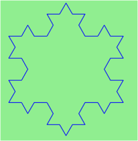
2. Modify the Koch fractal program so that it draws a Koch snowflake, like this:

   

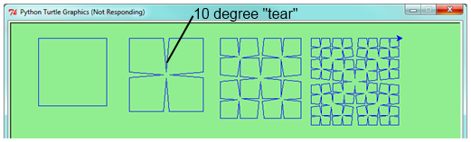
1. Draw a Cesaro torn square fractal, of the order given by the user. A torn square consists of four torn lines. We show four different squares of orders 0,1,2,3. In this example, the angle of the tear is 10 degrees. Varying the angle gives interesting effects — experiment a bit, or perhaps let the user input the angle of the tear.

   

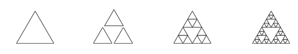
1. A Sierpinski triangle of order 0 is an equilateral triangle. An order 1 triangle can be drawn by drawing 3 smaller triangles (shown slightly disconnected here, just to help our understanding). Higher order 2 and 3 triangles are also shown. Adapt the Koch snowflake program to draw Sierpinski triangles of any order input by the user.

   

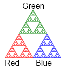
2. Adapt the above program to draw its three major sub-triangles in different colours, as shown here in this order 4 case:

   

3. Create a module named seqtools.py. Add the functions encapsulate and insert_in_middle from the chapter. Add tests which test that these two functions work as intended with all three sequence types.

4. Add each of the following functions to seqtools.py:

   def make_empty(seq): pass
   def insert_at_end(val, seq): pass
   def insert_in_front(val, seq): pass
   def index_of(val, seq, start=0): pass
   def remove_at(index, seq): pass
   def remove_val(val, seq): pass
   def remove_all(val, seq): pass
   def count(val, seq): pass
   def reverse(seq): pass
   def sort_sequence(seq): pass
   
   def testsuite():
       test(make_empty([1, 2, 3, 4]), [])
       test(make_empty(('a', 'b', 'c')), ())
       test(make_empty("No, not me!"), '')
   
       test(insert_at_end(5, [1, 3, 4, 6]), [1, 3, 4, 6, 5])
       test(insert_at_end('x', 'abc'),  'abcx')
       test(insert_at_end(5, (1, 3, 4, 6)), (1, 3, 4, 6, 5))
   
       test(insert_in_front(5, [1, 3, 4, 6]),   [5, 1, 3, 4, 6])
       test(insert_in_front(5, (1, 3, 4, 6)),   (5, 1, 3, 4, 6))
       test(insert_in_front('x', 'abc'),        'xabc')
   
       test(index_of(9, [1, 7, 11, 9, 10]), 3)
       test(index_of(5, (1, 2, 4, 5, 6, 10, 5, 5)), 3)
       test(index_of(5, (1, 2, 4, 5, 6, 10, 5, 5), 4), 6)
       test(index_of('y', 'happy birthday'), 4)
       test(ndex_of('banana', ['apple', 'banana', 'cherry', 'date']), 1)
       test(index_of(5, [2, 3, 4]), -1)
       test(index_of('b', ['apple', 'banana', 'cherry', 'date']), -1)
   
       test(remove_at(3, [1, 7, 11, 9, 10]), [1, 7, 11, 10])
       test(remove_at(5, (1, 4, 6, 7, 0, 9, 3, 5)), (1, 4, 6, 7, 0, 3, 5))
       test(remove_at(2, "Yomrktown"), 'Yorktown')
   
       test(remove_val(11, [1, 7, 11, 9, 10]), [1, 7, 9, 10])
       test(remove_val(15, (1, 15, 11, 4, 9)), (1, 11, 4, 9))
       test(remove_val('what', ('who', 'what', 'when', 'where', 'why', 'how')),
             ('who', 'when', 'where', 'why', 'how'))
   
       test(remove_all(11, [1, 7, 11, 9, 11, 10, 2, 11]),  [1, 7, 9, 10, 2])
       test(remove_all('i', 'Mississippi'), 'Msssspp')
   
       test(count(5, (1, 5, 3, 7, 5, 8, 5)), 3)
       test(count('s', 'Mississippi'), 4)
       test(count((1, 2), [1, 5, (1, 2), 7, (1, 2), 8, 5]), 2)
   
       test(reverse([1, 2, 3, 4, 5]), [5, 4, 3, 2, 1])
       test(reverse(('shoe', 'my', 'buckle', 2, 1)), (1, 2, 'buckle', 'my', 'shoe'))
       test(reverse('Python'), 'nohtyP')
   
       test(sort_sequence([3, 4, 6, 7, 8, 2]),  [2, 3, 4, 6, 7, 8])
       test(sort_sequence((3, 4, 6, 7, 8, 2)),  (2, 3, 4, 6, 7, 8))
       test(sort_sequence("nothappy"), 'ahnoppty')
   

   As usual, work on each of these one at a time until they pass all the tests.

   But do you really want to do this?

   Disclaimer. These exercises illustrate nicely that the sequence abstraction is general, (because slicing, indexing, and concatenation is so general), so it is possible to write general functions that work over all sequence types. Nice lesson about generalization!

   Another view is that tuples are different from lists and strings precisely because you want to think about them very differently. It usually doesn’t make sense to sort the fields of the julia tuple we saw earlier, or to cut bits out or insert bits into the middle, even if Python lets you do so! Tuple fields get their meaning from their position in the tuple. Don’t mess with that.

   Use lists for “many things of the same type”, like an enrollment of many students for a course.

   Use tuples for “fields of different types that make up a compound record”.

5. Write a function, recursive_min, that returns the smallest value in a nested number list. Assume there are no empty lists or sublists:

   test(recursive_min([2, 9, [1, 13], 8, 6]), 1)
   test(recursive_min([2, [[100, 1], 90], [10, 13], 8, 6]), 1)
   test(recursive_min([2, [[13, -7], 90], [1, 100], 8, 6]), -7)
   test(recursive_min([[[-13, 7], 90], 2, [1, 100], 8, 6]), 13)
   

6. Write a function count that returns the number of occurences of target in a nested list:

   test(count(2, []), 0)
   test(count(2, [2, 9, [2, 1, 13, 2], 8, [2, 6]]), 4)
   test(count(7, [[9, [7, 1, 13, 2], 8], [7, 6]]), 2)
   test(count(15, [[9, [7, 1, 13, 2], 8], [2, 6]]), 0)
   test(count(5, [[5, [5, [1, 5], 5], 5], [5, 6]]), 6)
   test(count('a', [['this', ['a', ['thing', 'a'], 'a'], 'is'], ['a', 'easy']]), 5)
   

7. Write a function flatten that returns a simple list containing all the values in a nested list:

   test(flatten([2, 9, [2, 1, 13, 2], 8, [2, 6]]), [2, 9, 2, 1, 13, 2, 8, 2, 6])
   test(flatten([[9, [7, 1, 13, 2], 8], [7, 6]]), [9, 7, 1, 13, 2, 8, 7, 6])
   test(flatten([[9, [7, 1, 13, 2], 8], [2, 6]]), [9, 7, 1, 13, 2, 8, 2, 6])
   test(flatten([['this', ['a', ['thing'], 'a'], 'is'], ['a', 'easy']]),
                 ['this', 'a', 'thing', 'a', 'is', 'a', 'easy'])
   test(flatten([]), [])
   

8. Rewrite the fibonacci algorithm without using recursion. Can you find bigger terms of the sequence? Can you find fib(200)?

9. Write a function named readposint that uses the input dialog to prompt the user for a positive integer and then checks the input to confirm that it meets the requirements. It should be able to handle inputs that cannot be converted to int, as well as negative ints, and edge cases (e.g. when the user closes the dialog, or does not enter anything at all.)

10. Use help to find out what sys.getrecursionlimit() and sys.setrecursionlimit(n) do. Create several experiments similar to what was done in infinite_recursion.py to test your understanding of how these module functions work.

11. Write a program that walks a directory structure (as in the last section of this chapter), but instead of printing filenames, it returns a list of all the full paths of files in the directory or the subdirectories. (Don’t include directories in this list — just files.) For example, the output list might have elements like this:

    ['C:\Python31\Lib\site-packages\pygame\docs\ref\mask.html',
     'C:\Python31\Lib\site-packages\pygame\docs\ref\midi.html',
     ...
     'C:\Python31\Lib\site-packages\pygame\examples\aliens.py',
     ...
     'C:\Python31\Lib\site-packages\pygame\examples\data\boom.wav',
     ... ]

12. Write a program named litter.py that creates an empty file named trash.txt in each subdirectory of a directory tree given the root of the tree as an argument (or the current directory as a default). Now write a program named cleanup.py that removes all these files. Hint: Use the program from the example in the last section of this chapter as a basis for these two recursive programs. Because you’re going to destroy files on your disks, you better get this right, or you risk losing files you care about. So excellent advice is that initially you should fake the deletion of the files — just print the full path names of each file that you intent to delete. Once you’re happy that your logic is correct, and you can see that you’re not deleting the wrong things, you can replace the print statement with the real thing.