Visualizing Logic Circuits - Introduction
This project is an outgrowth of two other very early Python-for-Fun projects: Logic Circuits and Logic Cirucuits two. These are still accessible and draw a fair following of readers. In those projects you have the ability to build digital logic circuits with primitive components and encapsulate a circuit into a component that can be used (even multiple times) in a more elaborate circuit. In those projects we ended up building one circuit to add binary numbers and another to multiply.
This project is similar but with a somewhat different focus.
- Components are drawn on a canvas, laid out relative to each other and connected with wires.
- The circuits contain a graphic representation of their components. This is drawn on the canvas using Pygame.
- Instead of more complex basic components such as the DFlipFlop, everything in this project is built from 2 input Nand gates and inverters, 3 types of switches, connectors and wires. By the end we will build a complete 4-bit binary counter.
- The display of the circuits may be zoomed in and out, through different layers of circuitry.
- The circuits run in an animation where the high and low signals in the wires are displayed by changing the color of each wire. Combined with the zoom lens it is much easier to see how everything works together.
- Most everything is object oriented and each component or circuit class also has a test class which creates the demo for this write-up.
The amount of code is a bit on the high side, but still, I think it will be very approachable. There are about 500 lines of code that build and animate components and circuits. Another 200 lines are in the test classes. But there is also a lot of repetition of the basic ideas.
It's good if you can have pygame installed so that you can follow along by actually running the programs and using the inputs rather than just watching the animations run. But even if not the screen-shots here should enable you to understand everything.
We will look at the basic components, and then combine them into small circuits. When drawn, circuits can be encapsulated which makes them look and act like basic components. Within an encapsulated circuit there are other components, including, perhaps, inner circuits.
Each component within a circuit resides in a layer. The layer is assigned automatically and is one more than its parent circuit. The top circuit resides in layer one.
When we view an animation we specify the layer depth to which we will view. Any circuit at this depth will be shown as a box. Circuits above this value will be shown expanded. Basic components at or above (i.e. lower layer numbers) will also be drawn as well as the wires connecting everything. Components and circuits in higher (deeper) layers are not drawn but they are still running.
Along with components we have connectors. Each basic component has a fixed number of connectors with names (like A,B,C). Wires run between connectors, linking a single output to zero or more inputs. Like basic components, circuits also have connectors that link their output and inputs to their internal connectors.
A Word about Pygame and Running the Programs
The code has been written using Python 2.7 and Pygame was easily available and downloaded for Windows 7 (download and run a .msi file) and for Ubuntu 12.04 (use apt-get install pygame). It has not been tested on the Macintosh and has not been tested on Python 3. Pygame itself has dependancies for generating the graphics. With the above 2 options these are handled automagically.
In this tutorial the programs are run from the command prompt ('$') supplying arguments after the program name. If you are using IDLE or another enviroment you will probably first input the command line arguments and then run the appropriate program.
Basic Components
In its current form the components that are "built-in" are the 2 input NAND gate, the INVERTER, and 3 kinds of switches. From these basic parts we'll build simple circuits and later we'll encapsulate circuits into components to be used in even more complex circuits.
The INVERTER is treated as a seperate component, but it could be easily made from a two input NAND gate by simply connecting both inputs to the same source. An Inverter has one input and one output and inverts the input signal at the output.
The NAND gate has two inputs and an output. The little circle on its output means that the output is calculated as an AND of the inputs and then inverted. Inversion is important. Without it we couldn't build most of what we be showing, especially memory circuits.
This is how actual electronic gates work. The INVERTER does nothing more than simply change a high to a low or a low to high. In electronic gates high is usually 5 volts and low is 0 volts. In this program high is red and low is blue.
Here is our first circuit that already uses four of the five basic components.

N1 is a NAND gate whose output (C) is low (blue) only if both inputs (A and B) are high (red). The inputs of N1 are controlled by switches. S1 is a simple toggle switch. Each time it is clicked it turns either off or on which makes the wire connecting it to input A of the Nand gate (N1.A) either blue or red (low or high). MP1 is a multi-pulsar. If clicked on it produces a stream of pulses, a signal that alternates between high and low. Clicked again returns it to its rest state (high).
The INVERTER I1 simply produces an output (B) which is the opposite of its input (A).
N1 and I1 together in this configuration form an AND gate whose output is high (red) if and only if both inputs are high. Though we won't be using basic AND gates in this project, it's nice to see how one can be built as a circuit. The AND gate also has its own symbol which is like the NAND but without the small circle on the right that indicates inversion.
As long as S1 is on (output is red), then whatever is produced by MP1 will be duplicated at I1's output. If S1 is clicked off however, the AND circuit will not pass on the signal from MP1. This is how an AND gate can work as a gateway. To run this in python use the command:
$ python basics.py layer=2
When the canvas appears like the window above click MP1 to start a pulse stream going. Then toggle S1 to see how the signal from MP1 is either stopped or passed through. Close the graphics window to exit the program.
Animated (return with the browser's Back button)
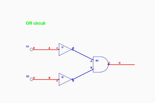
The next circuit uses 2 INVERTER gates feeding a NAND. This circuit forms the equivalent of an OR gate. The output of the NAND (connector N1.C) is high if either or both of inputs (the outputs of switches S1 and S2) are high.
Notice that in both the AND and OR circuit, two single inversions cancel each other out, resulting in positive logic. Here are two images one with both input low and another with one input high. Run it with the command:
$ python or.py layer=3
Again click on s1 and s2 to toggle them. Notice the output on the right is red if either of the two input switches on the left are red. As before, exit by clicking the X in the upper left corner of the graphics window.
Expanded OR circuit animated (return with the browser's Back button)
You might have noticed something else about the above screen shots. You have probably noticed that there is a fair amount going on in the representation of the circuit. The NAND, switches and INV's are all positioned and have labels (N1,I2,S1,S2) as do at least some of the connectors (A,B,C). We'll get into how all this is done later when we discuss the code.
Encapulating a Circuit
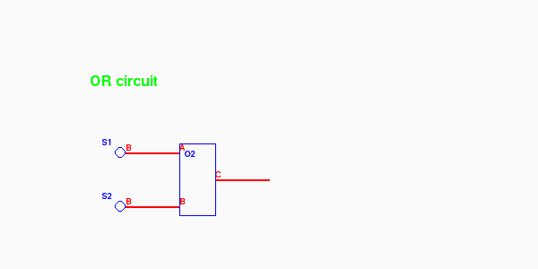
The test program or.py encapsulates the OR circuit onto layer 2. We can view through layer 1 onto layer 2 by passing the command line argument "2" we see the following:
$ python or.py layer=2
Encapsulated OR circuit animated (return with the browser's Back button)
Notice the labeling on the connectors. The boxed OR gate has inputs "A" and "B". The switches don't have input labels (it's just you and the mouse) but they do each have a "B" output connector.
Something a bit more complex
An XOR gate (exclusive or) outputs high if one and only one input is high. Here's another way to look at it. The output is high if the inputs are different. Below is a circuit using 4 NAND gates to provide this function on connector N4.C.
$ python xor.py layer=3

Animated (return with the browser's Back button)
The program xor.py encapsulates the 4 NAND gates into a circuit component on layer 2. Since we viewed through to layer 3 we peeked into the circuit inside the encapsulation. But if we look just through to layer 2 we see instead:
$ python xor.py layer=2

Animated (return with the browser's Back button)
Just like the AND gate, the OR gate and the XOR gate each has its own standard drawing form and it's NOT a rectangular box. But we won't be using these 3 gates further so I didn't spend any time on how they look. However, the flip-flops that now follow are all traditionally drawn as a box.
Flip-flops
The Simple Latch
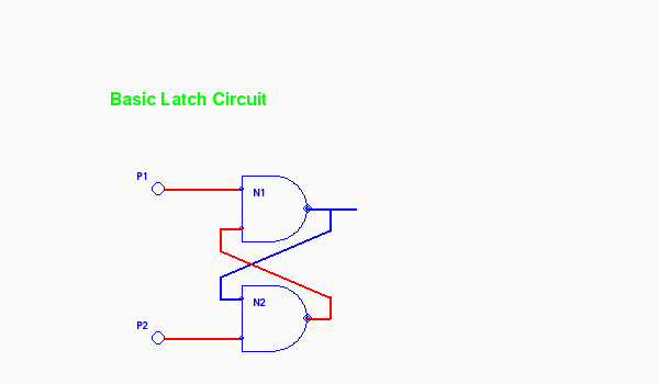
In the earlier logic projects we built a simple latch from 2 NAND gates. This demonstrated how positive feedback could be used to remember (store) data. Here is a simple latch:
$ python latch.py layer=3
Animated (return with the browser's Back button)
Pulsars P1 and P2 each issue a short single pulse to low when clicked and then return to high. The 2 NAND gates form a one-bit memory unit that basically remembers which pulsar was last clicked. Click them one after another and watch the output change. If this is new for you then spend some time studying the circuit to understand why it works as it does. The crossed wires provide that positive feedback. The circuit is quite symmetrical.
Encapulated the circuit looks like:
$ python latch.py layer=2

Animated (return with the browser's Back button)
The inputs on the left of the encapsulation box are generally labeled A and B and the output on the right is labeled Q (not C) and is fed from the output N1.C
When it is clear (generally from the geometry) I'm going to avoid labeling every input and output.
The Data Latch
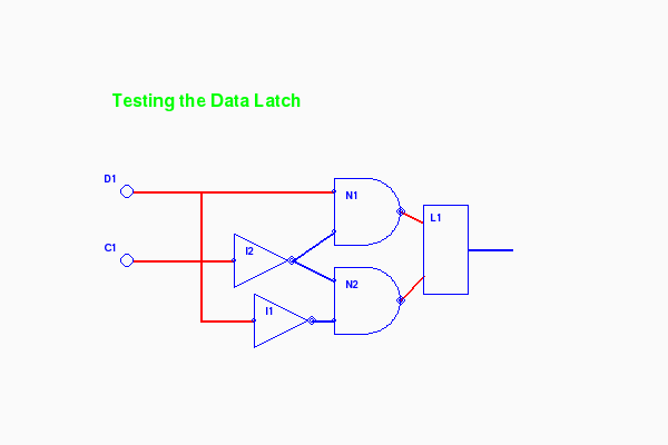
The simple latch above is not often used by itself because we usually want to do something else: We'll typically have a data line with a signal coming in and we want the ability to clock the signal value at a given point in time. By adding some front-end logic we can have exactly that: a circuit with two inputs (data and clock) and one output with the remembered value:
$ python dlatch.py layer=3
Animated (return with the browser's Back button)
Let's take a minute to study this. The data coming in from the switch D1 (a simple toggle switch) is delivered to both N1 and N2 but because of the inverter I1 it is delivered at opposite polarity. Switch C1 is a one-shot pulsar delivering a short downward pulse when clicked. I2 makes this an upward pulse to both N1 and N2. One of the outputs (either N1.C or N2.C) then drops setting the simple latch L1. When C1's pulse is over and its output returns to high, The data has been captured in L1.
We can also set the view all the way into layer 4 to see the workings of L1 as well:
$ python dlatch.py layer=4

Animated (return with the browser's Back button)
There's going to be a (not so) small problem, however. While the clock line is active (low), any change on the data line will be immediately be passed through to the output. This may or may not be serious depending on the application. For us it is a catastrophe because we will be using even more feedback from higher level outputs back to higher level inputs.
There is a way around this though. But we have to keep going.
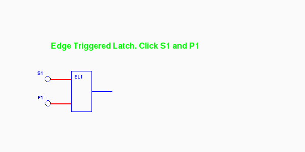
Edge Triggered Data Latch
Our next circuit works something like an airlock. The idea is simple. Don't let the air (or signal) rush through when the door is open. Use two doors. Open the second only after the first is closed.
The simple Data latch is like that single door and when the clock is low that door is opened just letting all that signal out. Our improved E-latch will use 2 D-latches and with a single inverter their 2 clock inputs can be exactly out of step. When one is open the other is closed.
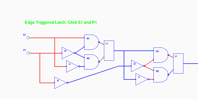
Here are three screen shots viewing through to layers 2, 3, and 4. The view to layer 3 is probably the most informative:
$ python elatch.py layer=2
Animated (return with the browser's Back button)
$ python elatch.py layer=3

Animated (return with the browser's Back button)
$ python elatch.py layer=4
Animated (return with the browser's Back button)
This reminds me a bit of using the zoom feature on map programs.
The Divide by Two Circuit
By adding just one inverter, we can turn an E-latch into a circuit with just one input (the clock) and convert a pulse stream on the input to another on the output with exactly half the frequency.
By feeding the output back to the data input inverted, the output will flip to the opposite polarity each time a pulse come in on the clock. More precisely, the output will flip each time the input clock goes from low to high. This creates a new pulse stream on the output with exactly half the frequency of the input pulse stream. Here is what it looks like at layer 3:
$ python div2.py layer=3

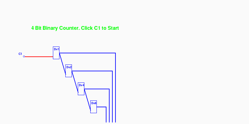
The Four Bit Binary Counter
By simply stringing four div2 circuits together the outputs become bits in a binary counter. Here's what the circuit looks like at layer 3:
$ python counter.py layer=3 scale=1
Animated (return with the browser's Back button)
The circuit consists of a multipulsar C1 and four Divide-by-2 components (DV1, DV2, DV4, DV8).
Notice that there are now 2 arguments on the command line. The first is still the layer to view. The second is a scale factor that determines the size of components drawn to the screen. This defaults to "2". But specifying "1" we get a half scale. Sometimes "3" and "4" are used as well to magnify the circuit.
The screen shot was taken while the counter was in operation. At the bottom the blue lines represent '1' bits, the red lines '0'. We caught the count at '0101' or in decimal 5.
The counter counts up to '1111' and then wraps back to '0000'. And if we take the red lines for '1' instead of blue, we have a counter that counts down to zero and then wraps back to 15 decimal.
Design Concepts
Settings
The module settings.py contains constants and also extracts scale and layer variables from the command line. Constants include colors we use as RGB tuples, screen dimensions, animation speed and parameters for the single and repeating pulse switches.
Component Abstract Class
The component class component.py is an abstract class. Basic component classes (Nand2, Inv, Swt) inherit this class as well as the circuit class. Component contains the attributes that all the sub-classes have in common such as name, position, layer and scale. Also common methods such as position alignment, handling mouse clicks, scaling of segments when drawing components. Sub-classes do not define their own __init__ method but must define a setupGraphics method which is called at the end of Component.__init__ and which will complete the initialization of the instance.
Basic Gates and Switches
The module gates.py contains the classes for the 2 input NAND gate (Nand2), the INVERTER gate and the the 3 types of switches. Each has a standard set of methods.
The setupGraphics methods make connectors to attach to the drawing. The self.output connector is mandatory as it's the source of a wire tree (more coming) that will disperse the output signal of the gate to appropriate input connectors on other gates.
The draw methods contain a list of arguments to use with pygame drawing commands. These arguments must be scaled before used to draw polygons, circles, etc.
Every component must have a computeOutput method which calculates the gate's output from its inputs and sometimes its history. Flip-flop circuits and pulse generators contain history.
The switches also have a takeClick method to respond to being clicked by the mouse.
Connectors
Connectors connector.py have several things in common with components but there are enough differences to make subclassing unattractive. Both have a parent, a name, a position, a value and a layer. Components have connectors for their inputs and output. The component is the parent of these connectors and they all reside in the same layer. For circuits that are encapsulated their external connectors reside one layer above the inner connectors.
Connectors connect to each other with wires. Interestingly, wires are not representated in the code. They are simply drawn during animation as a pygame line in either the HOT or COLD color from the source connector to one of its children its feed list.
Connectors may also reside independently within a circuit. In this case the circuit is the parent and both circuit components and these connectors reside in the same layer. These connectors make it easy to "fan out" a signal on a wire are even simply let a wire change direction.
Finally, external connectors in a circuit are used to connect the circuit-component into the rest of the circuit one layer up. These connectors reside in the layer above.
If a connectors parent has to move (scoot over), then the connector must also. The subject of alignment in circuit layout will be discussed below.
During construction of a circuit the method addWire connects components together. This method takes an arbitrary number of connector instances, or (x,y) positions as arguments. Each position argument creates a free standing connector named "Anon" at the x,y position. Method addWire works through the arguments left to right, and populates the feeds list of each connector appropriately. It returns the last connector as its function value, letting us chain these calls or fan a signal out quite easily.
During animation the method drawWires recursively walks the links between connectors and paints wires (lines) along the way. Since they are just wires all connected together, they all carry the same signal and are painted the same color.
Wires are not drawn inside an encapsulated circuit. This is controlled the the layer attribute of both the source and target. If either is hidden (below the visible viewing layer) then the wire is not drawn.
Usually, two "connected" connectors reside on the same layer. The exception is with a circuit's external connectors (at layer n) and its internal wiring (at layer n+1).
Also during animation the method sendOutput works much like drawWires. It transmits the signal from an output connector, through other connectors, on to input connectors on basic components. The difference is that, unlike drawWires, sendOutput doesn't stop at a hidden layer, but goes right to the bottom. The sendOutput method is defined for components as well as connectors.
Text Processing
Text (text.py) is used to label basic components and encapsulated circuits with their names, create banners and to optionally label connectors. Text is tied to a given x,y point and placed in one of four quadrants. When text.py is run stand-alone it creates a image that shows how the four quadrants are used:
$ python text.py
Alignment
Early versions of this project required me to carefully position each component of a circuit working out the x,y position by hand. The origin of a component or circuit is the upper left corner, basically the pygame convention. If a component is inside a circuit its x,y is relative to the origin of the circuit it is in.
When we start to scale, placing items by hand can quickly fall apart. What works much better is to place the first component at a fixed x,y position and then place other components relative to the first or to each other.
This is very effective if a circuit or component can align itself to another by specifying one of its own connectors and another connector from the target, along with an (x,y) offset between the connectors. This creates a very flexible system that adapts to scaling quite nicely. You've already seen this is the above screen shots. We want to use connectors because we run wires between them and this makes it easy to space components easily and also to have wiring that is largely horizontal or vertical.
The methods align and scootOver make this work. If a circuit is aligning itself to another it will scoot over appropriately and all the bits inside (components, connectors, subcircuits) must scoot over too. This is the sort of situation that can make recursion fun. We'll be seeing more of this now as we start to examine some of the code in detail.
A Walk through some Code
A Simple Animation
Let's have another look at our first circuit.
Here is the Python code to build and then animate it:
# basics.py
#  Show off the basic gates in a simple circuit
#
from   gates     import MultPuls, Nand2, Inv, Swt
from   circuit   import Circuit

class TestBasic1 (Circuit) :
    def setupGraphics(self) :
        self.banner = "Basic components. Switch, Multipulsar, Nand, Inverter"

        n1 = Nand2(self,"N1", self.scale1((50, 30))) # Nand Gate
        i1 = Inv  (self,"I1")            # Inverter
        s1 = Swt  (self,"S1")            # Switch feeding input A
        m1 = MultPuls (self,"MP1")       # Pulsar feeding input B

        s1.align(s1.B, n1.A, -50, 0)  # line up the gates
        m1.align(m1.B, n1.B, -30, 0)
        i1.align(i1.B, n1.C,  80, 0)  # inverter follows Nand

        n1.A.labelQuad = 2            # Label all connectors
        n1.B.labelQuad = 2
        n1.C.labelQuad = 1
        i1.A.labelQuad = 2
        i1.B.labelQuad = 1

        self.gates = (m1,s1,n1,i1)
        s1.B.addWire(n1.A)
        m1.B.addWire(n1.B)
        n1.C.addWire(i1.A)
        i1.B.addWire( (i1.B.x(30), i1.B.y()))  # tail to see

if __name__ == "__main__" :
    import gameloop
    from   settings import CmdScale
    circuit = TestBasic1 (None, "TestBasic1",(100,100),scale=CmdScale)
    gameloop.gameloop(circuit)
Let's explain what is going on. The program can run stand-alone with the module name "__main__". The gameloop animation expects to be passed a circuit to animate (at bottom) so we define a class for our circuit and build an instance of it. This is a subclass of Circuit inheriting all of the standard code and we supplement it with the method setupGraphics which is automatically called from __init__ in the abstract Component class. An instance of TestBasic1 is built in the second to last line and then passed to the gameloop.py for animation.
The setupGraphics method defines the 2 gates and 2 switches and sets the banner attribute. Only the Nand gate is given a position of (50,30) scaled and offset relative to its parent, the pygame screen. The Inverter and 2 switches are created with a default position (0,0) and then align themselves to the Nand gate. Switch s1 aligns its output connector 50 units to the left of the Nand's A input (N1.A). The inverter I1 aligns its input 80 units to the right of N1's output connector(N1.C). A unit here is one pixel times the scale factor. The scale factor defaults to two.
The connectors are all assigned a labelQuad attribute to have their labels printed in the appropriate quadrant. The circuit self is assigned a gates attribute. This is a list of its components and used by the abstract Circuit class in the methods computeOutput, checkClicked and draw. (see circuit.py). And finally, wires are created connecting the two switches to the Nand, the Nand to the Inverter and then a piggy tail wire just to show the final output from the Inverter.
Circuits
The Circuit class circuit.py lets us combine components and optionally encapsulate them into a single component with its own connectors to the outside world. Circuits made for encapsulation (put into a box) do not have switches or banners and typically we don't label the interior connectors. On the other hand the outermost (top) circuit is generally never encapsulated and it so makes sense to have switches among its components and to label it more fully.
The Circuit class is quite small and enables the animation of a circuit with the following
- The method computeOutput for a circuit simply calls the same for each component in its gates attribute as well as sendOutput which distributes the signals within the circuit. The order of computation and distribution is set by the order of the components in gates
- The method checkClicked simply passes asks each of its components to do the check for the being clicked and repsond. This is only in the top non-encapsulated circuit.
- The draw method provides 3 possibilities.
- The circuit may be hidden and not drawn at all if it resides below the viewing layer.
- The circuit may be drawn as a box with just a label and external connectors if it exactly on the viewing layer.
- The circuit may be drawn in detail if it is above the viewing layer.
A Fuller Example
Let's return to the OR circuit or.py and look at the code. This will be the only module we'll study in detail. All the later circuits follow exactly the same pattern.
The first part of the setupGraphics method looks like:
class Or (Circuit) :
  def setupGraphics(self) :
      n1 = Nand2(self,"N1", self.scale1((80, 30))) # Nand Gate
      i1 = Inv  (self,"I1") # Inverter for n1.A
      i2 = Inv  (self,"I2") # Inverter for n1.B
      i1.align(i1.B, n1.A, -40, -20)  # inverter precedes Nand
      i2.align(i2.B, n1.B, -40,  20)  # inverter precedes Nand
      # external connectors
      self.A = Connector(self,"A",((i1.A.x(-20),i1.A.y() )))
      self.B = Connector(self,"B",((i2.A.x(-20),i2.B.y() )))
      self.C = Connector(self,"C",((n1.C.x( 20),n1.C.y() )))
      self.output = self.C       # who is output

      # child gates for computeOutput and draw methods
      self.gates = (i1,i2,n1)
      # for convenience let internal gates be seen from outside
      self.i1,self.i2,self.n1 = (i1,i2,n1)
We define the 3 gates with the circuit self as the parent. The first one n1 is set at a scaled position in the circuit. The two inverters i1 and i2 are defined and then aligned to n1. The exteral connectors A, B, and C are built and placed at a (x,y) position relative to the internal gates. These positions are used if the circuit is drawn in detail. The output is identified as connector C. The gates attribute is constructed. The individual gates are also kept as attributes of the circuit. This allows them to be referenced from outside the circuit itself (only sometimes a good idea):
continued ....
      # internal connectors
      i1.B.addWire(n1.A)
      i2.B.addWire(n1.B)
      # connect external connectors to internal components
      self.A.addWire(i1.A)
      self.B.addWire(i2.A)
      n1.C.addWire(self.C)

      if self.encapsulated() :  # if encapsulated re-work externals
          self.A.pos, self.B.pos, self.C.pos = self.scaleM((0,5),(0,35),(20,20))
The rest of setupGraphics method does the wiring between connectors both internally and to the 3 external external connectors self.A, self.B and self.C. So now, if the circuit is displayed in detail these 3 external connectors are in position to be wired into the circuit above. If the circuit is shown encapsulated (as a box) then these connectors need to take new positions that align to the box.
Next we have test circuit whose purpose is simply to instantiate and Or circuit and test it by adding switches, a banner and what not. In this case we labeled all of the connectors both inside (like or2.n1.A) and outside (like s1.B). Here is the code for that:
class TestOr (Circuit) :
  def setupGraphics(self) :
      self.banner = "Encapsulated OR circuit"
      or2 = Or(self,"O2"  , self.scale1((50,30)))
      s1 = Swt  (self,"S1")   # Switch feeding input A
      s2 = Swt  (self,"S2")   # Switch feeding input B

      s1.align(s1.B, or2.A, -30, 0)  # line up the gates
      s2.align(s2.B, or2.B, -30, 0)
      s1.B.addWire(or2.A)
      s2.B.addWire(or2.B)
      s1.B.labelQuad = 1
      s2.B.labelQuad = 1
      self.gates = (s1,s2,or2)

      or2.n1.A.labelQuad = 3            # Label all the connectors
      or2.n1.B.labelQuad = 2
      or2.n1.C.labelQuad = 1
      or2.i1.A.labelQuad = 2            # Inverter
      or2.i1.B.labelQuad = 1
      or2.i2.A.labelQuad = 3            # Inverter
      or2.i2.B.labelQuad = 4
      or2.A.labelQuad = 1
      or2.B.labelQuad = 1
      or2.C.labelQuad = 1
      or2.C.addWire( (or2.C.x(30), or2.C.y()))  # tail to see
Finally, or2.py is meant to be run as main. When it is invoked from the command line the scaling factor and view layer are taken from sys.argv or the defaults in the settings module settings.py. Then a TestOr instance is created, which further creates an Or instance along with the surroundings to test it. The TestOr instance is passed to the gameloop function:
if __name__ == "__main__" :
  import gameloop
  from   settings import CmdScale
  circuit = TestOr (None, "TestOr",(100,100),scale=CmdScale)
  gameloop.gameloop(circuit)
This same pattern is used in the modules that stack like nested russian dolls. Once you understand one, the others are easy.
latch.py, dlatch.py, elatch.py, div2.py, counter.py.
Each one of these can be run stand-alone from the command line as we have seen.
The gameloop
When one of the stand-alone modules is run as main it builds its test circuit and passes it to the gameloop function in gameloop.py. The latter is short and pretty much boiler plate Pygame. It creates a screen and enters an event loop. The constant TICKS_PER_SECOND in the settings module specifys how rapidly the loop is run.
Within the loop a few things happen. A mouse click on the window termination button will shut the program off. A mouse click on a switch (or pulsar) will toggle it. The switch itself is found by a recursive search through layers of circuits (generally not very deep) using the mouse coordinates. Next, the circuit is asked to compute its output, a request that also is sent recursively through the tree of circuits producing signals sent through wires at all layers. The screen is then erased and the circuit is drawn, wires and all. The draw request is also sent recursively through the circuits. Finally, the screen is flipped and the process repeats. At the default setting of 200 times a second.
All of the code files can also be obtained as logicPygame.zip
A Final Note
This project has been a lot of work but also a lot of fun. Much of the effort has been spent on extending the functionality of the program when new ideas came along, but doing it in a way that did not increase the code size nor disrupt the structure. Rewriting large parts of the code was quite common.
I had thought earlier that rewriting this code in Javascript would be worthwhile to demonstrate the circuits dynamically. But the animated GIFs work just as well and it's better to stay in Python. Pygame has been used in another Python for Fun project, the updated Lode Runner video game.
If you have comments or suggestions You can email me at mail me
Copyright © 2015-2018 Chris Meyers